Certification
I hereby certify that this project work was carried out by OBASA OLORUNFEMI OLUWANISOLA of the Department of Water Resources Management & Agrometereology, Federal University of Agriculture, Abeokuta under the guidance and supervision in accordance with the standard required by the Department of Water Resources Management & Agrometereology.
| Signatory | Role | Signed |
|---|---|---|
| Dr. Grace O. Oluwasanya | Project Supervisor | 13/8/12 |
| Prof. N. J. Bello | Head of Department | 13/8/12 |
| – | External Supervisor | – |
Acknowledgements
It would not have been possible to write this thesis without the help and support of the kind people around me, to only some of whom it is possible to give particular mention here. Above all, I would like to thank my wonderful parents and Beautiful sisters for their unequivocal support throughout, as always, for which my mere expression of thanks likewise does not suffice.
This thesis would not have been possible without the help, support and patience of my supervisor, Dr. Grace O. Oluwasanya, her advice and unsurpassed knowledge of Water Safety Management has been invaluable on both an academic and a personal level, for which I am extremely grateful.
I would like to acknowledge the academic and technical support of the Laboratory technologists; Mr. Abulumein, Mrs. J.A Fashina, Mr. Adesuyi and Ms. Dadagbon as their patience in answering my numerous queries was not in vain. I also thank the Department of Water resources Management and Agrometereology for their support and assistance since the start of my undergraduate programme, especially the Head of department, Prof. N. J. Bello.
I am most grateful to Dr. Z. O, Ojekunle, Dr. G.C Ufoegbune, Pastor and Mrs. Emesibe, Pastor A. Daramola, Pastor (Dr.) C. Adejuyigbe, Mr. and Mrs. O. Kuyinu, Prof. Ozojie, and countless more, for their timely inspirations, assistance and positive criticisms.
I would like to thank Mr. Mayowa Ojo for his kindness, friendship and support, together with the other officers of Ogun-Osun River Basin Development Authority (OORBDA). I remember the encouragement of Theophilus, who graced me with the privilege of his friendship all the way from Liberia.
Amongst my colleagues in the Department of Water resources Management, the efforts made by Adefarati Adekunle and Adeyemo Adeola to mention a few in promoting a stimulating and welcoming academic and social environment that will stand as an example to those that succeed them. I would also like to thank my colleagues and friends scattered in other departments of this great Institution.
Last, but by no means least, I thank my friends in Abeokuta, Lagos, and elsewhere for their support and encouragement throughout, some of whom have not been named for their desire to remain incognito. Thanks for believing, even when I stopped believing.
For any errors or inadequacies that may remain in this work, of course, the responsibility is the author's.
Abstract
Climate change poses uncertainties to the supply and management of water resources. The Intergovernmental Panel on Climate Change (IPCC) estimates that the global mean surface temperature has increased by 0.6 ± 0.2 °C since 1861, and predicts an increase of 2 to 4 °C over the next 100 years. Temperature increases also affect the hydrologic cycle by directly increasing evaporation of available surface water and vegetation transpiration. These climatic changes can influence precipitation amounts, timings and intensity rates, and indirectly impact the flux and storage of water in surface and subsurface reservoirs (i.e., lakes, soil moisture, and groundwater). In addition, there may be other associated impacts, such as sea water intrusion, water quality deterioration and potable water shortage amongst others. While climate change affects surface water resources directly through changes in the major long-term variables such as air temperature, precipitation, and evapotranspiration, the relationship between the changing climate variables and groundwater is more complicated and poorly understood. This study examined climatic (rainfall and temperature) and water quality data of the last two decades to establish the presence of climate change (if any) and possible impacts using Abeokuta South Local Government Area as Case Study. The water quality parameters examined were pH and Nitrates. A strong correlation (r² = 99.3% and 97.9) was observed between rainfall and Nitrate content as well as pH. The study concluded that Climatic variation has its impacts on NO₃ and pH, though it is difficult to predict what dimensions the impacts might take in the future.
Keywords: Climate change; Groundwater quality; Shallow wells.
CHAPTER ONE: INTRODUCTION
Water is indispensable for life, but its availability at a sustainable quality and quantity is threatened by many factors, of which climate plays a leading role. The Intergovernmental Panel on Climate Change (IPCC) defines climate as "the average weather in terms of the mean state and its variability over a certain time-span and a certain area". Climate change is a statistically significant variation of the mean state of the climate or of its variability lasting for decades or longer. Evidence is mounting that we are in a period of climate change brought about by increasing atmospheric concentrations of greenhouse gases. Atmospheric carbon dioxide levels have continually increased since the 1950s. The continuation of increasing atmospheric concentrations may significantly alter global and local climate characteristics, including temperature and precipitation. Climate change can have profound effects on the hydrologic cycle through precipitation, evapotranspiration, and soil moisture with increasing temperatures. The hydrologic cycle will be intensified with more evaporation and more precipitation. However, the extra precipitation will be unequally distributed around the globe. Some parts of the world may see significant reductions in precipitation or major alterations in the timing of wet and dry seasons Information on the local or regional impacts of climate change on hydrological processes and water resources is becoming more important. The effects of global warming and climatic change require multi-disciplinary research, especially when considering hydrology and global water resources (Kumar, 2010).
Global sea levels have risen between 10 and 25 cm since the late 19th century. As a direct consequence of warmer temperatures, the hydrologic cycle will undergo significant impact with accompanying changes in the rates of precipitation and evaporation. Predictions include higher incidences of severe weather events, a higher likelihood of flooding, and more droughts. The impact would be particularly severe in the tropical areas, which mainly consist of developing countries, including Nigeria. Changes in regional temperature and precipitation have important implications for all aspects of the hydrologic cycle. Variations in these parameters determine the amount of water that reaches the surface, evaporates or transpires back to the atmosphere, becomes stored as snow or ice, infiltrates into the groundwater system, runs off the land, and ultimately becomes base flow to streams and rivers.Hydrological impact assessments of watersheds (and aquifers) require information on changes in evapotranspiration because it is a key component of the water balance. However, climate-change scenarios tend to be expressed in terms of changes in temperature and precipitation. Consequently, the effects of global warming on potential evaporation (or more inclusively, evapotranspiration) are not simple to estimate. Many global scenarios suggest an increase in potential evaporation, but these factors may be outweighed locally or regionally by other factors reducing evaporation. Various models may be used to calculate potential evaporation using data on net radiation, temperature, humidity, and wind speed, and sometimes plant physiological properties. The estimated effect of a change in climate on potential evaporation depends on the characteristics of the site.
According to Kumar, (2010), Water resource management plans increasingly need to incorporate the effects of global climate change to accurately predict future supplies. Numerous studies have documented the sensitivity of stream flow to climatic changes for watersheds all over the world. Most of these studies involve watershed scale hydrologic models, of which validation remains a fundamental challenge. Moreover, outputs from general circulation models (GCM) can be rather uncertain and downscaling their predictions for local hydrologic use can produce inconsistent results. Therefore, the sensitivity of stream flow to climate changes is perhaps best understood by analyzing the historical records. Building empirical models to link climate and regional hydrological regimes has a long history. In recent years, many researchers have used empirical rainfall-runoff model to study the impacts of climatic change on hydrology. However, applications of these empirical relationships to climate or basin conditions different from those used in the original development of these functions are questionable. Although the most noticeable impacts of climate change could be fluctuations in surface water levels, the greatest concern of water managers and government is the potential decrease of the quality and quantity of groundwater supplies, as it is the main available source of potable water supply for human consumption and irrigation of agricultural produce worldwide. As groundwater aquifers are recharged mainly by precipitation or through interaction with surface water bodies, the direct influence of climate change on precipitation and surface water ultimately affects groundwater systems.
It is increasingly recognized that groundwater cannot be considered in isolation from the landscape above, the society with which it 'interacts or from the regional hydrological cycle, but needs to be managed holistically. In understanding the likely consequences of possible future (climate and non-climate) changes on groundwater systems and the regional hydrological cycle, an important (but not exclusive) component to understand is the influence that these factors exert on recharge and runoff. It is important to consider the potential impacts of climate change on groundwater systems. As part of the hydrologic cycle, it can be anticipated that groundwater systems will be affected by changes in recharge (which encompasses changes in precipitation and evapotranspiration), in the nature of the interactions between the groundwater and surface water systems, and changes in use related to irrigation (Kumar, 2010).
Determining the potential impact of climate change on groundwater resources, in particular, is difficult due to the complexity of the recharge process, and the variation of recharge within and between different climatic zones. When considering water resources in coastal zones, coastal aquifers are important sources of freshwater. However, salinity intrusion can be a major problem in these zones. Salinity intrusion refers to replacement of freshwater in coastal aquifers by saltwater. It leads to a reduction of available fresh groundwater resources. Changes in climatic variables can significantly alter groundwater recharge rates for major aquifer systems and thus affect the availability of fresh groundwater. Salinisation of coastal aquifers is a function of the reduction of groundwater recharge and results in a reduction of fresh groundwater resources. A link between rising sea level and changes in the water balance is suggested by a general description of the hydraulics of groundwater discharge at the coast. Fresh groundwater rides up over denser, salt water in the aquifer on its way to the sea (Figure 1-1), and groundwater discharge is focused into a narrow zone that overlaps with the intertidal zone. The width of the zone of groundwater discharge measured perpendicular to the coast, is directly proportional to the discharge rate. The shape of the water table and the depth to the freshwater/saline interface are controlled by the difference in density between freshwater and salt water, the rate of freshwater discharge and the hydraulic properties of the aquifer. The elevation of the water table is controlled by mean sea level through hydrostatic equilibrium at the shore.
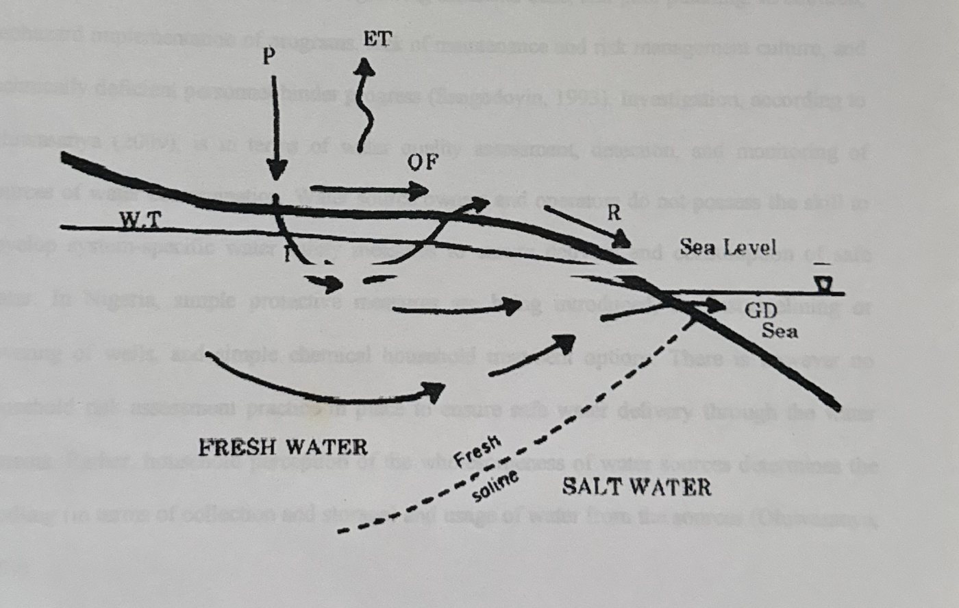
1.1 The National Context of the Research
The research area is in Nigeria, West Africa. According to Oluwasanya (2009), The Nigerian Government has made considerable investment in water supply programs (JMP, 2006), yet, 53% of the 140 million people have no access to potable water and safe drinking systems (JMP, 2008). One reason for such a high percentage is the rapid population growth that has not been accompanied by an increase in the delivery of essential services like water supply. It was estimated that in 2008 only about 65% of the urban and 30% of the small towns' population have access to reliable water supply of acceptable quality (JMP, 2008). The overall effective urban water supply coverage may be as low as 30% of the total population due to poor maintenance and unreliability of supplies (WBR, 2005). Rural water supply coverage is estimated at 30% (JMP, 2008); Oluwasanya (2009). The other reasons given for the inadequacies in safe water delivery include the limited investment in the sector despite rapid socio-economic rate of development, a growing industrial base, and poor planning. In addition, haphazard implementation of programs, lack of maintenance and risk management culture, and technically deficient personnel hinder progress (Sangodoyin, 1993). Investigation, according to Oluwasanya (2009), is in terms of water quality assessment, detection, and monitoring of sources of water contamination. Water source owners and operators do not possess the skill to develop system-specific water safety measures to ensure delivery and consumption of safe water. In Nigeria, simple protective measures are being introduced, for instance lining or covering of wells, and simple chemical household treatment options. There is however no household risk assessment practice in place to ensure safe water delivery through the water systems. Rather, household perception of the wholesomeness of water sources determines the handling (in terms of collection and storage) and usage of water from the sources (Oluwasanya; 2009)
1.2 The Study Area
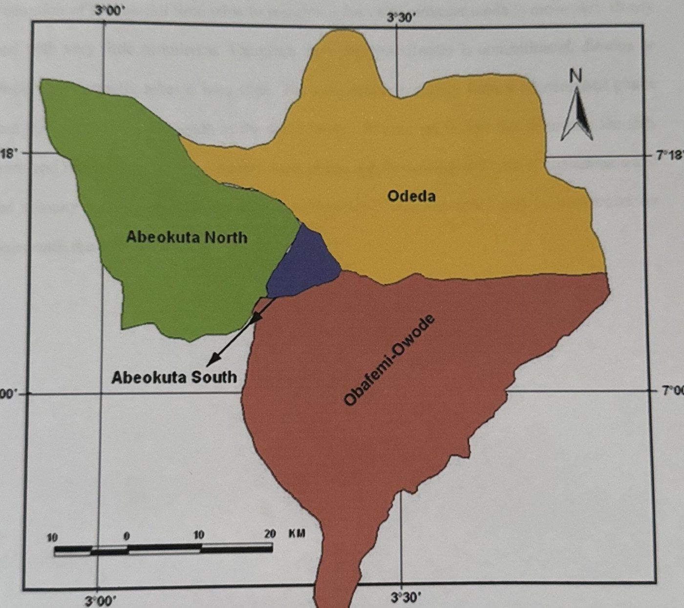
The research area is Abeokuta, the capital city of Ogun State in south-western Nigeria. Oluwasanya (2009) described Abeokuta as an ancient township that is gradually being transformed into a modern urban city. The city has about 250,000 people inhabiting more than 50 heterogeneous townships (Onakomaiya et al., 1992). Abeokuta is in the humid tropics with seven - eight months of bi-modal peak rainy season and an average annual rainfall of 1,200 mm. The area is underlain by the crystalline Basement Complex consisting of igneous and metamorphic rocks. Groundwater however occurs in the fractured and in-situ weathered portion of the rocks (Martins et al., 2000).
1.3 Groundwater and Climate Change
As a result of rapid expansion of cities and subsequent population explosion, the development of groundwater resources for potable use has increased substantially over the last decade especially in developing countries.
Close relationship exists between groundwater quality and climate change. Various changes in climatic conditions can result in ground water contamination. Potential sources of groundwater contamination through climate change could include change in air temperatures, disruption of the rainfall time table to mention a few. Groundwater tends to move very slowly and with very little turbulence. Therefore once the groundwater is contaminated, dilution or dispersion normally takes a long time. The contaminants usually form a concentrated plume that flows along the same path as the groundwater. Among the factors that determine the size, form and rate of movement of contaminant plume are the amount and type of contaminant and the velocity of groundwater movement. Groundwater contaminants could be undetected for years until the supply is topped for use.
1.4 Aim of the Research
The Aim of this research is to understand the implications of climate change (if any) on water quality of Self- supply Systems in Abeokuta, Nigeria through the following; 1. Assessment of climatic conditions (precipitation and temperature) in the study area between 1990 and 2011. Assessment of Self-Supply Systems water quality variation (physical, chemical and microbiological) with climatic data in the study area between 1990 and 2011. 3. Identification and classification of climatic impacts (if any) on the quality on Self-Supply Systems within the study areas. 4. Assessment of current water quality status of Self-supply Systems. 5. Identification of existing adaptation strategies of self-supply water quality management. 6. Recommendation of appropriate adaptation approaches to water quality management.
1.5 Problem statement
The impacts of Climate Change on the quality of self-supply Systems in Abeokuta South Local Government Area of Ogun state are poorly understood.
1.6 Justification of the Research
Climate change is a global phenomenon which impacts on life and most natural processes and resources. Water, its quality and management is no doubt one of those processes. Water is the single most abundant resource on the face of planet earth however, it is not readily available. Groundwater resources and their long-term replenishment are controlled by longterm climate conditions. Hence, Climate change will have a great impact on groundwater resources.Groundwater is likely to play an even greater role for human development under changing climatic conditions especially in developing countries such as Nigeria. "Although the effects of climate change on groundwater resources are not adequately understood at present, they cannot be ignoredạồIPCC 1998, p. 122)
1.7 Thesis Outline and Structure
The thesis is sub-divided into six (6) chapters. They are the introduction in chapter 1, literature review (chapter 2), research area (chapter 3), and the research methods captured in chapter 4.
Chapter 5 presents the results and discussion of the research findings. It sets the scene for the research discussions. The chapter provides the background and the underlying argument, which shaped the structure of the research results and discussions sections. Summaries of findings, the implication of research outcomes to water quality, and appropriate recommendations are presented within each results section.
Chapter six contains the concluding part of the thesis. The chapter reiterates the research objectives and summarises the major research findings. It further presents an integrated discussion reflecting the implication of research outcomes for implementation within the research and the wider context.
CHAPTER TWO: LITERATURE REVIEW
This chapter explores and captures as much as possible the background knowledge around groundwater and Climate Change. The chapter in addition explores related topics such as groundwater resources in terms of water quality and contamination. Finally, the chapter highlights some knowledge gaps in relation to the research objectives.
2.1 Water on Earth
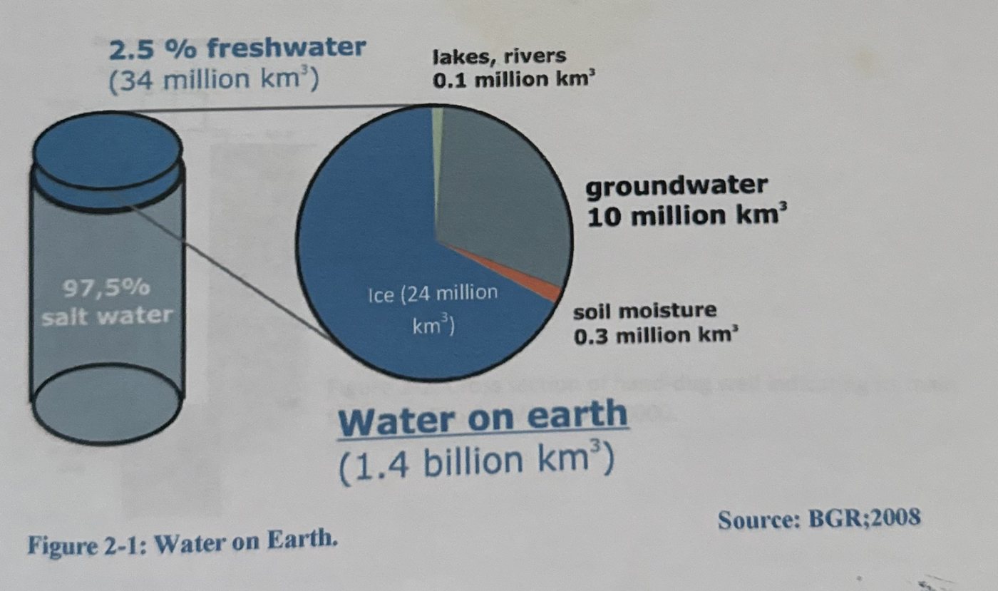
On a global scale, one third of the world's population depends on groundwater for their drinking water, in urban as well as rural areas. In arid and semi-arid areas, the dependency on groundwater for water supply is between 60 and 100%. The importance of groundwater has been marginalized and often neglected in many development strategies and projects. Therefore, the aim of halving the number of people without sustainable access to safe drinking water and basic sanitation (Millennium Development Goal, MDG 7) depends very much on how ground water resources are developed and managed (BGR; 2008).
2.2 Shallow wells
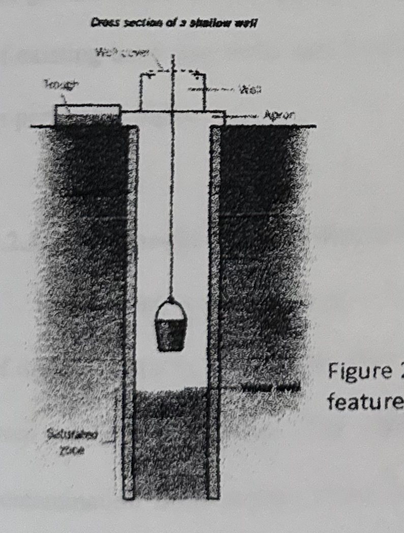
Hand-dug wells can be described as excavations with diameters large enough to accommodate one or more men with shovels digging down to below the water table; Hand-dug wells can be lined with laid stones or brick; extending the lining upwards above the ground surface to form a wall around the well which serves to reduce both contamination and injuries by falling into the well.
2.2.1 Dimensions of Hand-dug wells
Depths of Hand-dug wells range from shallow wells, about 5 metres deep, to deep wells over 20 metres deep; (IT Publications, 1985). Wells with depths over 30 metres are sometimes constructed to exploit an aquifer. It is impractical to evacuate a well which is less than a metre in diameter, an excavation of about 1.5 metres provides adequate working space for the diggers and will allow a final internal diameter of about 1.2 metres after the well has been lined (1T Publications, 1985).
A more modern method called caissoning uses reinforced concrete or plain concrete pre-cast well rings that are lowered into the hole. (Figure 2-2)
A well-digging team digs under a cutting ring and the well column slowly sinks into the aquifer, whilst protecting the team from collapse of the well bore. Hand dug wells provide a cheap and low-tech solution to accessing groundwater generally in rural locations in developing countries. Hand-dug wells may be built with a high degree of community participation, or by local specialized artisans who specialize in hand-dug wells.
2.2.2 Mode of operation
Generally, the well water is operated by an electric submersible pump, a trash pump, a vertical turbine pump, a hand-pump or a mechanical pump (e.g. from a water-pumping windmill. Water can also be drawn up using containers, such as buckets that are raised mechanically or by hand. Wells can vary greatly in depth, water volume and water quality. Well water typically contains more minerals in solution than surface water. Hand dug wells have low operational and maintenance costs, in part because water can be extracted manually, without a pump. Hand dug wells can be easily re-dug or deepened, which may be necessary if the ground water level drops, by telescoping the lining further down into the aquifer. The yield of existing hand dug wells may be improved also by deepening or introducing vertical tunnels or perforated pipes.
2.2.3 Drawbacks to Hand-dug wells
Drawbacks to Hand-dug wells are numerous, include but not limited to; impracticality of digging wells in areas where hard rock is present, it can be time-consuming to dig and line even in favorable areas. The wells are susceptible to yield fluctuations and possible contamination from surface water, including sewage. Hand dug well construction generally requires the use of a well-trained construction team, and the capital investment for equipment such as concrete ring molds, heavy lifting equipment, well shaft formwork, motorized dewatering pumps, and fuel can be large for people in developing countries. Construction of hand dug wells can be dangerous due to collapse of the well bore, falling objects and asphyxiation, including from dewatering pump exhaust fumes. Household water treatment however, allows households to take responsibility for their own water quality. The personal incentive to improve one's own supply also brings direct benefit (Sutton, 2005).
2.3 Groundwater Quality
Ground waters are generally free of suspended solids and objectionable odor. In some instances however, the water may be associated with underground beds of peat and decaying vegetation, which contribute substantial amount of Colour -producing organic matter to the supply, (Murdoch et al. 2000). Interactions between atmospheric, terrestrial, and aquatic processes in a watershed as well as the human use of resources affect water quality. Climate change will influence the components of the identified processes leading to direct and indirect changes in water quality, (Murdoch et al. 2000). There is usually no contamination of groundwater by sewage or industrial wastes except in fissured aquifers where surface pollution may be easily transmitted to the groundwater reservoir. Contamination may also result from the use of reclaimed wastes to recharge groundwater supplies. The temperature of ground water is a highly describable characteristic for cooling and other purposes. Groundwater is uniformly cool and usually has a temperature near the long term average air temperature for the region. It is common for deeper ground water to show increasing temperature with increasing depth. (Kilanko; 1995). Water Quality guidelines are however given for various uses of drinking, irrigation, livestock watering, industries and a host of other uses by the World Health Organization (WHO). Individual countries may also have guidelines of water quality that is peculiar to them.
2.4 Groundwater Contamination
Groundwater contamination occurs when man-made products such as gasoline, oil, road salts and chemicals get into the ground water and cause it to become unsafe and unfit for human use. Some of the major sources of these products, called contaminants, are storage tanks, septic systems, hazardous waste sites, landfills, and the widespread use of road salts, fertilizers, pesticides and other chemicals.
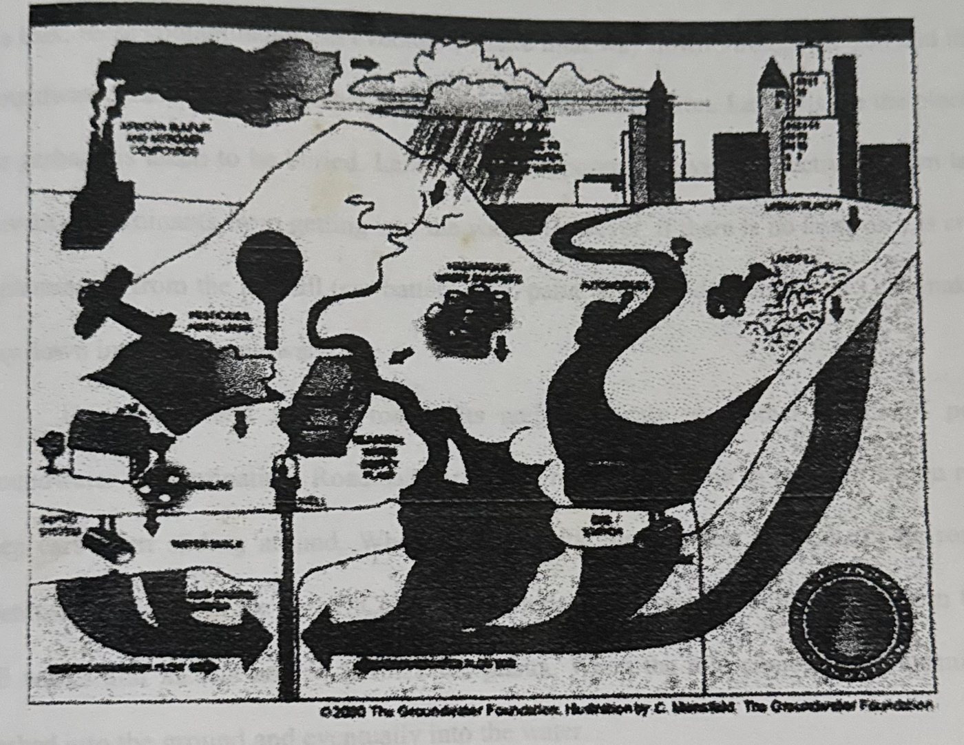
2.4.1 Sources of Groundwater Contamination
Storage tanks may contain gasoline, oil, chemicals, or other types of liquids and they can either be above or below ground. If the contaminants leak out and get into the groundwater, serious contamination can occur. Septic systems can be another serious contamination source.
Septic systems are used by homes, offices or other buildings that are not connected to a city sewer system. Septic systems are designed to slowly drain away human waste underground at a slow, harmless rate. An improperly designed, located, constructed, or maintained septic system can leak bacteria, viruses, household chemicals, and other contaminants into the groundwater causing serious problems. Hazardous waste sites can lead to groundwater contamination if there are barrels or other containers laying around that are full of hazardous materials. If there is a leak, these contaminants can eventually make their way down through the soil and into the groundwater. Landfills are another major source of contamination. Landfills are the places that our garbage is taken to be buried. Landfills are supposed to have a protective bottom layer to prevent contaminants from getting into the water. However, if there is no layer or it is cracked, contaminants from the landfill (car battery acid, paint, household cleaners, etc.) can make their way down into the groundwater.
The widespread use of road salts and chemicals is another source of potential groundwater contamination. Road salts are used in the wintertime to put melt ice on roads to keep cars from sliding around. When the ice melts, the salt gets washed off the roads and eventually ends up in the water. Chemicals include products used on lawns and farm fields to kill weeds and insects and to fertilize the plants. When the rain comes, these chemicals get washed into the ground and eventually into the water.
2.5 Contamination indicators
Groundwater contamination indicators are examined under three sub-headings. These are non-microbial parameters, microbiological indicators and nitrate as groundwater pollution indicator. The indicators that are of interest to this research are discussed within the relevant headings.
2.5.1 Non-microbial Parameters
Temperature
Temperature is a physical property of matter that quantitatively expresses the common notions of hot and cold. Objects of low temperature are cold, while various degrees of higher temperatures are referred to as warm or hot (Wikipedia, 2012). The most physical assessment of water quality is the measurement of temperature. Temperature impacts both the physical and biological characteristics of surface water. It affects the photosynthesis of aquatic plants, metabolic rates of aquatic organisms and the sensitivity of these organisms to pollution, parasites and diseases. Increased amounts of sediments in water absorb heat from sunlight rather than reflect it. This causes the temperature of water to rise.
pH
pH is a measure of the activity of the (solvated) hydrogen ion. p[H], which measures the hydrogen ion concentration is closely related to, and is often written as, pH. Pure water has a pH very close to 7 at 25°C. Solutions with a pH less than 7 are said to be acidic and solutions with a pH greater than 7 are basic or alkaline. The pH scale is traceable to a set of standard solutions whose pH is established by international agreement. Primary pH standard values are determined using a concentration cell with transference, by measuring the potential difference between a hydrogen electrode and a standard electrode such as the silver chloride electrode. Measurement of pH for aqueous solutions can be done with a glass electrode and a pH meter, or using indicators. W.H.O standard for pH is 6.5 - 8.5.
Electrical Conductivity
Electrical conductivity is a measure of the capacity of water to conduct an electrical current and is a function of the types and quantities of dissolved substance in water. As concentration of dissolved ions increase, conductivity of the water increases. Specific conductance is the conductivity expressed in units of Micro siemen per centimeter at 25°C Specific conductance is a good surrogate for total dissolved solids and total ions concentrations, but there is no universal linear relation between total dissolved solids and specific conductance. Rather, the relation between specific conductance and constituent must be determined for each site. A continuous record of specific conductance can be used in conjunction with chemical analyses and continuous discharge records to estimate constituent loads. W.H.O standard for conductivity: 1000ms/cm.
Total Dissolved Solids
Total Dissolved Solids (often abbreviated as TDS) is a measure of the combined content of all inorganic and organic substances in a liquid in: molecular, ionized or microgranular (colloidal soil) suspended form. Generally, the operational definition is that the solids must be small enough to survive filtration through a sieve the size of two micrometers (Wikipedia 2012). Total dissolved solids are normally discussed only for freshwater systems, as salinity comprises some of the ions comprises some of the ions constituting the definitions of TDS. Primary sources for TDS in receiving waters are Agricultural and residential run-off, leaching of soil contamination, point source water pollution, discharge from industrial or sewage treatment plants. W.H. O standard for Total Dissolved Solids is 500mg/l.
2.5.2 Microbiological indicators
Microbiological Indicators refer to the number and types of organisms that inhabit water. The poorer the quality of water, the fewer the number and types of organisms that can live in it (Wheeling Jesuit University; 2004). The microbial indicators discussed below are however those of interest to this research, namely Escherichia coli and Clostridium perfringens.
Table 2-1: Criteria for microbial indicators
- The indicator should be absent in unpolluted water and present when the source of pathogenic microorganism of concern is present
- The indicator should not multiply in the environment
- The indicator should be present in greater numbers than the pathogenic microorganisms
- The indicator should respond to natural environmental conditions and water treatment processes in a manner similar to the pathogens of concern
- The indicator should be easy to isolate, identify and enumerate.
- The test should be inexpensive thereby permitting numerous samples to be taken
- The indicator should not be a pathogenic microorganism (to minimise the health risk to analysts).
The coliform groups consist of several genera of bacteria belonging to the family Enterobacteriaceae. Total and fecal coliform are differentiated by incubating at different temperatures (44.5°C for fecal and 35°C for total) and by using slightly different media broths. The total and fecal coliform bacteria test is a primary indicator of "Potability", suitability for consumption, of drinking water. It measures the concentration of total coliform bacteria associated with the possible presence of disease causing organisms.
Coliform bacteria are a natural part of the microbiology of the intestinal tract of warm blooded mammals, including man. Coliform bacteria can also be found in soil, other animals, insects, etc. The total coliform group is relatively easy to culture in the lab, and therefore, has been selected as the primary indicator bacteria for the presence of disease causing organisms.
Potential Health Hazards
Coliform bacteria are not pathogenic (disease causing) organisms, and are only mildly infectious. For this reason these bacteria are relatively safe to work with in the laboratory. If large numbers of coliforms are found in water, there is a high probability that other pathogenic bacteria or organisms, such as Giardia and Cryptosporidium, may be present. The PADEP requires public drinking water supplies to demonstrate the absence of total coliform per 100 mls (about 4 oz.) of drinking water. At this time, there are no regulations governing individual water wells. It is up to the private well owner to have his or her water tested.
Relevance to Sustainable/Unsuitable Development
The concentration of fecal coliforms in freshwater bodies is an indirect indicator of contamination with human and animal excreta. Water contaminated with human and animal excreta poses a serious health risk and is therefore unsuitable for potable supply unless it has been suitably treated. Fecal indicator bacteria remain the preferred way of assessing the hygienic quality of water. Escherichia coli (E. coli), the thermo tolerant and other coliform bacteria, the fecal streptococci and spores of sulphite-reducing clostridia, are common indicators of this type used. This measure indicates situations where treatment is required or has to be improved to guarantee safety of supply. As population density increases and/or more people are provided from a supply, the more critical the supply of safe, potable water becomes.
Clostridium perfringens
Only a small fraction of the thousands of species of bacteria on the earth cause disease in humans. Bacterial infection can be prevented by killing bacteria with heat, as in sterilization and pasteurization. If a bacterial infection does occur, doctors may treat it with antibiotics. However, overuse of antibiotics in recent years has enabled the development of strains of bacteria that are resistant to antibiotics. E.g. Clostridium perfringenswhich causes Clostridialmyonecrosis (gas gangrene) (Microsoft Encarta 2009)
2.5.3 Chemical Contamination Indices
Chemical Attributes of water are important indicators. Chemical Attributes affect aesthetic qualities such as the appearance, odour, and taste. Chemical indices also affect toxicity and safety of water. Assessment of water quality by chemistry involves the measurement of many elements and molecules dissolved or suspended in water. Commonly measured chemical parameters include; pH, Alkalinity, Hardness, Nitrates, Nitrites and Ammonia, Ortho- and total phosphates, Dissolved Oxygen and Chemical Oxygen Demand.
Nitrate (NO₃)
Nitrogen is essential for all living things, as it is an essential component of protein. Nitrogen exists in the environment in many forms and changes forms as it moves through the nitrogen cycle.Nitrogen is the nutrient applied for lawn and garden care and crop production to increase productivity. Feedlots, animal yards, septic systems, and other waste treatment systems are additional sources of nitrogen that is carried in waste. Nitrogen occurs naturally in the soil in organic forms from decaying plant and animal residues. Bacteria in the soil convert various forms of nitrogen to nitrate, a nitrogen/oxygen ion. This is desirable since the majority of the nitrogen used by plants is absorbed in the nitrate form. However, nitrate is highly soluble and readily moves with water through the soil profile. If there is excessive rainfall or overirrigation, nitrate will drain below the plant's root zone and may eventually reach groundwater.
Nitrate in groundwater may result from point sources such as sewage disposal systems and livestock facilities, from nonpoint sources such as fertilized cropland, parks, golf courses, lawns, and gardens, or from naturally occurring sources of nitrogen. Proper site selection for the location of domestic water wells, including depth and upslope with adequate separation distances between wells and possible contamination sources, can reduce potential nitrate contamination of drinking water. Proper well construction and maintenance also reduces the risk of drinking water contamination. Nitrate in water is undetectable without testing because it is colorless, odorless, and tasteless.
Chloride
Almost all natural waters contain chloride ions. Their concentrations vary considerably according to the mineral content of the earth in any given area. In small amounts they are not significant. In large concentrations they present problems. Usually chloride concentrations are low. Low to moderate concentrations of chloride add palatability to water. In fact, they are desirable for this reason. Excessive concentrations of either, of course, can make water unpleasant to drink. The WHO Regulations recommend a maximum concentration of 250 mg/1 for chloride ions (expressed as CI). Chlorides give water a salty taste. In large concentrations chlorides cause a brackish, briny taste that definitely is undesirable. Although chlorides are extremely soluble, they possess marked stability. This enables them to resist change and to remain fairly constant in any given water unless the supply is altered by dilution or by industrial or human wastes. Chlorides contribute to the total mineral content of water. As indicated above, the total concentration of minerals may have a variety of effects in the home. High concentrations of chloride ions add to the electrical conductivity of water. Chlorides can be substantially removed from water by reverse osmosis. Deionization (demineralization) or distillation will also remove chlorides and sulfates from water, but these methods are less suitable for household use than reverse osmosis.
Hardness
Hardness of natural waters is caused largely by high mineral content (calcium and magnesium salts and to a small extent by iron, aluminum, and other metals). Hardness resulting from the bicarbonates and carbonates of calcium and magnesium is called temporary hardness and can be removed by boiling, which also sterilizes the water. The residual hardness is known as non-carbonate, or permanent, hardness (Microsoft Encarta 2009). Hard water is generally not harmful to one's health but can cause serious problems in industrial settings. In domestic settings, hard water is often indicated by lack of suds formation when soap is agitated in water. Wherever water hardness is a serious concern, water softening is commonly used to remove hard water's adverse effects.
2.6 Groundwater and Climate Prediction
The Global hydrological cycle is a central component of the earth's climate system. As Global warming amplifies the water holding capacity of the atmosphere, the frequency of very heavy rainfall events (that is those in the uppermost quantities of rainfall distribution) is projected to increase (Allen and Ingram, 2002; Trenberth et al.,2003; Pali et al., 2007). In the tropics, where the Study area lies, air temperature will lead to larger absolute rises in the moisture content of the atmosphere. Increase in rainfall intensities are expected to be especially pronounced. Strategies to adapt to more variable fresh water resource will in many environments increase groundwater abstraction.
2.7 Climate Change
Climate shift is occurring more rapidly than can be attributed to natural causes and significant impact to water supply and quality is expected (Wikipedia 2012).
2.7.1 Definition
Climate change is a significant & lasting change in the statistical distribution of weather patterns over periods (time) ranging from decades to millions of years regardless of the cause. Climate change can also be used to refer to change in climatic conditions caused by human activities as opposed to changes in climate that may have resulted as part of earth's natural processes. Evidence of climate change in climatic conditions includes but not limited to; temperature change, precipitation and change in sea level. Changes to patterns of precipitation will be one of the first and critical impacts; affecting water availability not just for Agriculture and industry, but also for the basic drinking water and domestic needs of populations in many areas. Precipitation changes will lead, and have already led to extended droughts. Changes will also include greater intensity of rainfall, which will increase erosion and the difficulty of capturing water for storage as well as wide variations in the timing of precipitation which will affect the reliability and quality of water supplies. While climate scientists do not yet know with certainty the full scope of the effects of climate change on the planet, or how fast these changes will occur, the clear consensus is that significant impacts to the environment will be felt in the coming century. There is also a growing awareness that the first and perhaps most critical impacts will be on the world's freshwater resources. The impacts are not theoretical; and are already being felt in many parts of Nigeria and other countries such as the United States. Climate change is affecting the quality and quantity of water availability for municipal supply, food production, power generation, industrial use and other vital services in many geographic locations, including areas that are not traditionally considered water-poor. The great variety and regional variability of potential impacts, and many uncertainties associated with predicting the severity of the impacts, compound the challenge of assessing and responding to climate change vulnerability. Climate provides fundamental limits on the opportunities for human activities and ecosystems functioning within a Geographical area. A changing climate could also lead to alterations in water supply, air, soil, and water quality; ecosystem health; human health, resource use and the economy. While controversy persists over the relative contribution of human activities to climate change, the basic science behind the greenhouse effect and the data showing a sharp climatological shift in recent decades are not controversial. Regional climate shifts can be relatively sudden and dramatic, suggesting that climate systems can reach a 'tipping point' of greatly accelerated change. Climate change may be limited to a specific area or region or occur globally.
2.7.2 Mechanisms of Climate Change
The mechanisms that are primarily responsible for climate change as well as the time it takes for their initial responses to manifest.
Internal mechanisms
When the initial forcing mechanism is internal, it simply means that the causal processes are irreversible and from within the earth whose initial response could take centuries or millions of years to manifest. Such irreversible processes may include but not limited to; solar output, volcanism, and shifting in plate tectonics.
External mechanisms
When the initial forcing mechanism is external, the causal processes may include; increase in carbon (iv) oxide levels due to Emission of greenhouse gases, Land use, Ozone depletion, Animal Agriculture, Deforestation, Aerosol use, and Cement manufacturing to mention a few. The initial response is faster e.g. the thermal expansion of ocean water, but a full response may take centuries. (Wikipedia; 2011)
The focus of the research is Climate change caused by external mechanisms as the initial measurable response is much faster than that of internal mechanisms.
2.7.3 Processes of Climate Change
Here, we will be highlighting the various processes that are (but not limited to) associated with climate change.
Over the past century, the global average temperature has increased by approximately 0.6°c. Among the most undisputed predictions of climate change research is that average temperatures, particularly over land, will continue to increase. Estimates of the magnitude of warming vary widely due to uncertainties in the models used to predict warming; however, the temperature increase is generally predicted to accelerate over the coming century. As reported in the intergovernmental panel on climate change (IPCC) fourth assessment report, (IPCC, 2007), 11 of the 12 warmest years in more than 150 years of instrumental records of global surface temperatures have occurred since 1995.
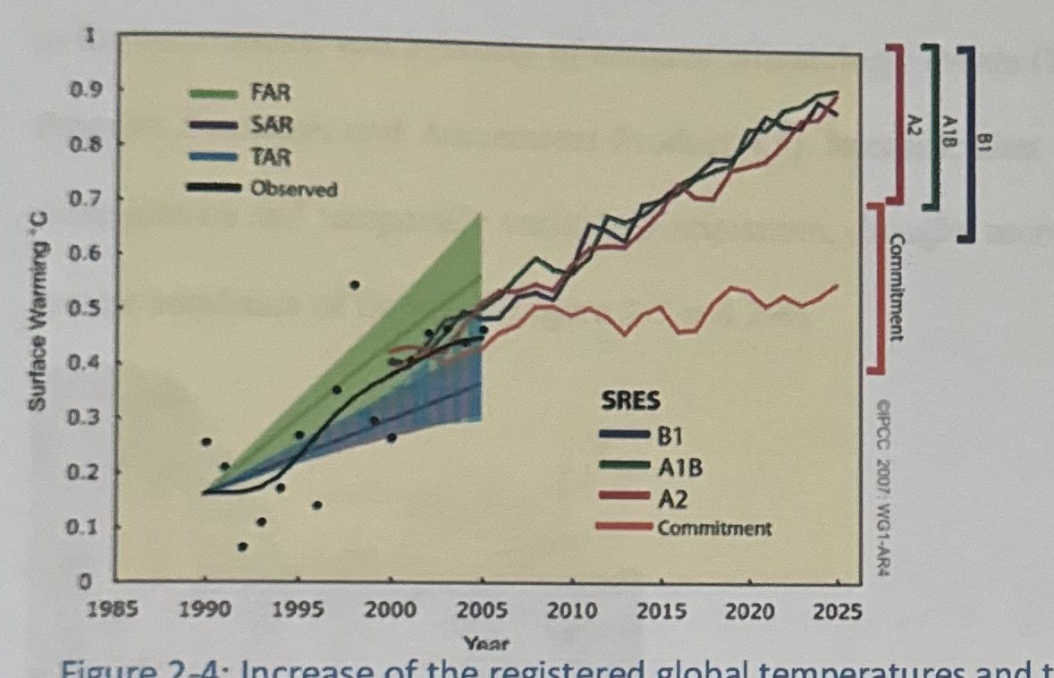
Increasing Evaporation and Precipitation
Another highly certain prediction of climate change research is that warmer temperatures will cause water to evaporate more readily, increasing total precipitation on a global scales. As with predictions of temperature increase, estimates of the magnitude of precipitation increase vary widely. It is generally accepted that the pattern of precipitation change will be highly complex and variable; some regions will receive more precipitation and other less than currently received.
Warmer temperature will contribute to sea level rise through melting of polar ice and expansion of water volume due to ocean warming. The IPCC reports that average global oceans temperatures have increased to depths of at least 3,000 meters (m) and that the ocean has been absorbing more than 80% of the heat added to the climate system. Estimates of the amount of sea level rise over the coming century range from 0.2m - 0.6m (IPCC, 2007)
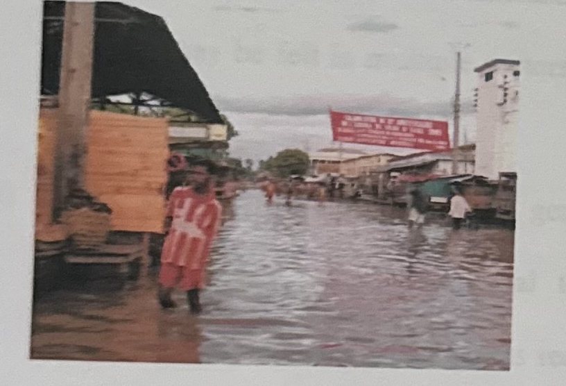
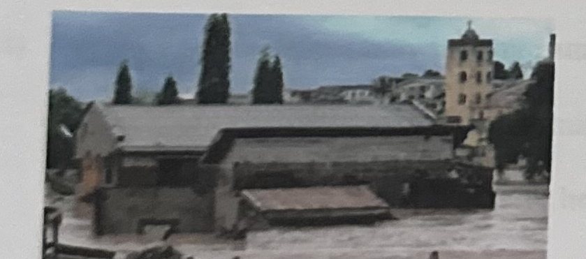
Climate change processes act to intensify the hydrologic cycle, leading to the increases in the occurrences and intensity of extreme climatologic events (U.S. Climate Change Science Program Synthesis and Assessment Product 4.3). Intensification is likely to be manifested by more intense and temporally variable precipitation, drought, more intense tropical storms, and greater incidence of flooding (Figure 2-5 and 2-6).
2.7.4 Climate Change Scenarios within the Study Area
In this section, an outline of the potential climate change within the study area in the aftermath of observed current global warming is attempted. While analyses were undertaken for several climatic parameters including cloud cover, precipitation, diurnal temperature range, minimum temperature, maximum temperature, average daily temperature and vapor pressure, only two of them namely precipitation and maximum temperature are discussed.
(i) The most significant changes are with respect to temperature and temperature related parameters. There has been a tendency to emphasize changes in temperature in the temperate latitudes and to imply that similar changes will not occur in tropical areas. Changes in minimum and maximum temperatures of the order of 7°C or more could be expected in certain parts of the country. This is likely to create a significantly different world with implications on vulnerability and adaptive capacity. The impacts of such changes may be felt in multiple sectors including: health, water, biodiversity, agriculture and forestry.
(ii) Night time temperatures may in general increase at a higher rate than day time temperatures. This has a potential to alter the themo-period to the detriment of biodiversity. Crops and other plants requiring low temperature conditioning may in the short run survive through autonomous adaptations, but in the long run, may suffer extinction.
(iii) Day time temperatures may in future attain levels unknown to areas outside the hot desert regions. In areas with perennially humid air, this has the potential to produce sultriness usually associated with the oppressive heat.
(iv) One aspect of the current climate pattern that will be carried forward into the potential climate of the future is zonation. All the parameter values are still likely to increase or decrease with distance from the coastline. Rainfall and humidity will decrease, while temperature will increase with distance from the sea.
(v) Uncertainties regarding climate change will most likely be in terms of magnitude rather than of direction. The more significant uncertainties pertain to temperature and temperature related parameters in respect of which the expected changes are relatively large. With respect to moisture, the projections are for an increase rather than a decrease.
The worst case scenarios are the situations in which the moisture level does not change (Drinking Water and Climate change; Special issue; 2008).
2.8 Research Issues: Introduction
2.8.1 Justification for Research Issues
The research asks a number of questions as follows:
- What is the impact of Climate change on the water quality provided through Self-supply systems?
The urban poor are, by and large, especially vulnerable to unreliable access from both public utilities and private and informal sources. Although State governments are ultimately responsible to see to it that everyone's human right to water is met, the urban poor is generally un-served by the water utilities and depend more on three other water sources: public standpipes (stand posts or fountains; sometimes in the form of communal taps); small-scale private water providers (vendors); and/or household or communal wells. Being un-served by the public system even though a water supply network may be in place, poor urban dwellers in particular have to meet their own needs. Self-supply by accessing water from own or shared wells is often the choice they make.
The other Questions are:
- What water quality parameters are associated with climate change?
- Through what pathways and mechanisms does Climate change affect Groundwater quality?
- What are the potential impacts of climate change on the “beneficial uses of water”?
- How do Identified Climatic Impacts vary across the study area
- What are the implications for decision-making?
- What are the key- impacts of a changing climate?
- What options are available for adaption to impacts of Climate change?
- How can climate change be incorporated into long-term planning and decisions in the study area?
2.9 Key Implications for Water Quality
Warmer water temperatures affect physical, chemical, and biological processes: As air temperature increases, water temperatures in rivers, streams, lakes, reservoirs, and ground water are also expected to mirror that rise. Warmer water temperatures reduce dissolved oxygen concentrations, which are a critical aquatic ecosystem requirement. Changes in rate of chemical reactions in the water column, sediment-water interface, and water-atmosphere interface are also expected. Aside the implications listed above, other such as below may arise.
- Taste and odor problems in drinking water may increase.
- Periods of thermal stratification may be extended with associated declines in dissolved oxygen.
- Changes in mixing depth affect productivity.
- Non-point source pollution increases with higher intensity precipitation events.
- Climate change may make it significantly more costly to meet water quality goals.
- Water quality remediation targets may not be met.
CHAPTER THREE: STUDY AREA
3.0 Introduction
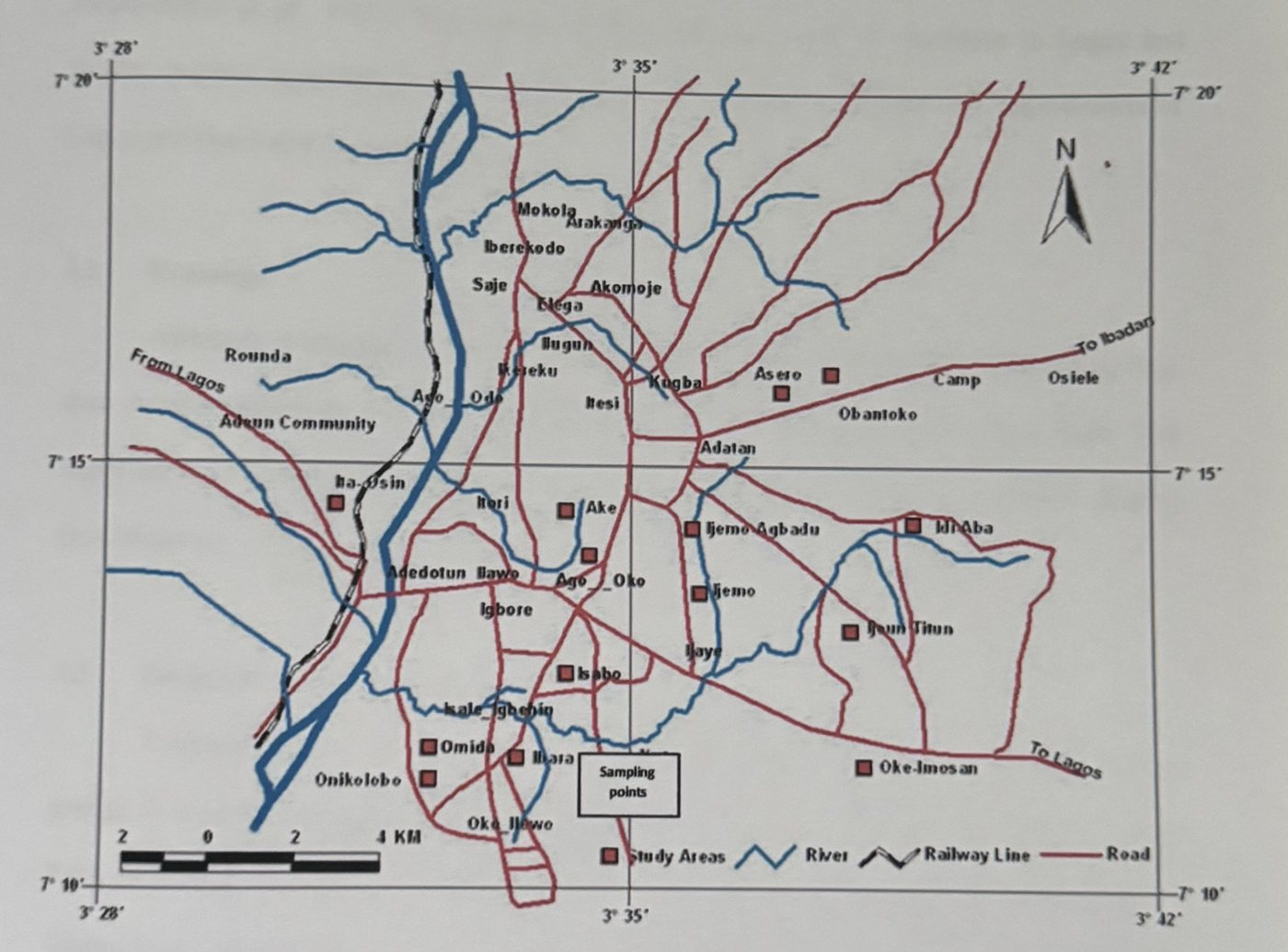
The study was carried out in urban and peri-urban areas of Abeokuta south local government in the capital of Ogun State, Nigeria (See Figure 3-1).
3.1 Demography and Socio-Economic Structures
Based on the 2006 national population survey, the city has 250,278 people inhabiting some 50 heterogeneous townships. Most of the people living within the city are engaged either in public and private employment or large and small scale business activities. The federal, state and local governments provide the formal type of employment. For instance about 89% of the federal government agencies are found within the city while virtually all the state public institutions and major banks in the country are either located or have branch offices in the city (Onakomaiya et al., 1992). The relative position and proximity of Abeokuta to Lagos and Ibadan, makes it accessible to these neighboring economically developed State capital cities of Lagos and Oyo State respectively.
3.2 Drainage
Abeokuta is drained by fast flowing coastal rivers flowing from the neighboring Oyo state through Abeokuta and emptying their contents into the lagoons in Lagos State. The important ones include Ogun and Shasha. River Ogun sometimes overflow its banks causing flood disasters.
3.3 Geography and Agriculture
Abeokuta lies in fertile country, the surface of which is broken by masses of grey granite. It is spread over an extensive area, being surrounded by mud walls 18 miles in extent. Palm-oil, timber, rubber, yams and shea-butter are the chief articles of trade. It lies below the Olumo Rock, home to several caves and shrines. The town depends on the Oyan River Dam for its water supply, which is not always dependable.
3.4 Geology
The state is underlain by two basic rock types, the crystalline (Basement complex) rocks and the sedimentary rocks, (Jones and Hockey, 1984). The Abeokuta formation extends throughout the whole width of the outcrop of sedimentary rocks and it thickens towards the west and dips towards the coast. It is over 250m thick near the border of the republic of Benin and 150m thick in the east. The formation is predominantly avenaceous and at the base with considerable thickness of clays, sands and shales of the continental marine origin. The uppermost layer is laterite which varies in thickness.Abeokuta is located at an altitude of approximately 157 m above sea level amidst isolated out-crops of natural formation of granitic rocks, which gives the city's landscape its undulating characteristics.
3.5 Vegetation and land use
There are two major physical features, which have exerted direct influence on the physical growth and development of the city. The first is the presence of Olumo rock (172.8 m) at the central part of the city. The other is the Ogun River located at the South-western part passing through the foot of Ashuwon hill. The physical features produced a unique pattern of landscape for the city and, to some extent, limited the physical growth and expansion of the city to the flatter and more easily developed terrain. Oyesiku and Kojeku (1992) noted that *Abeokuta, like most traditional urban centres in Nigeria, has continued to develop amorphously without conscious physical planning. In spite of its long years of existence, the city has no physical development plan (e.g. master plan) as different land uses compete rather than complement one another. The noted is largely a reflection of the city's traditional setting before and during the colonial administration.
CHAPTER FOUR: MATERIALS AND METHODS
This Chapter describes in detail the methods employed in the collection, examination, data analysis and the storage of the water samples. It also describes the statistical tools used in analyzing the data obtained from the laboratory.
4.1 Sample Design
Sample Design is the way or means of choosing the units of the study-individuals, Households, enterprises, communities, and societies etc., within the study area (Wikipedia; 2012). A recent map of the study area was obtained was from the Headquarters of the Local Goverment Area. The owners of the selected wells were visited to explain the purpose of the research and seek the permission for sampling and interviews. Future meetings were also scheduled on the same day. More than 120 self-supply wells were located within the study area, most of which are in use (Kyambade, 2006). With reference to the map, wells and boreholes were located and identified on the map of the study area (Figure 4-1). Households were visited once per month until the final samples were collected.
4.2 Initial Reconnaissance Survey
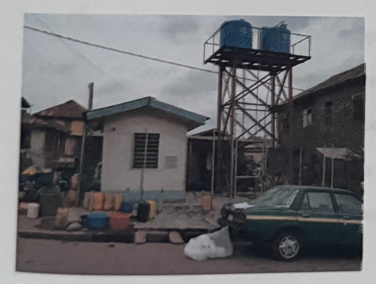
A survey of the study area allowed familiarization with the area (Taxi routes and shortcuts) for easy and rapid movement of samples between sample points and the laboratory. General observations in the sanitary environment e.g water supply and distribution systems e.g. pipes. (Where available) were noted.
4.3 Sample Collection
Sample collections were done on the 23rd of March, 4th of April and 10th of May, 2012. Water sampling in March was done 10 days after the Ist rains for the year had fallen. The First rain of the year fell on the 13th of March, 2012 (Field records). Samples were later stored at ambient temperatures, cool and dry. The kegs were first rinsed with the water sample for collection, filled to the brim with a bailer or tap (as the case may be), immediately sealed and labeled with paper tapes to prevent contamination and distortion with other samples. These were stored in a cool dry place after analysis.
4.4 Well Classification
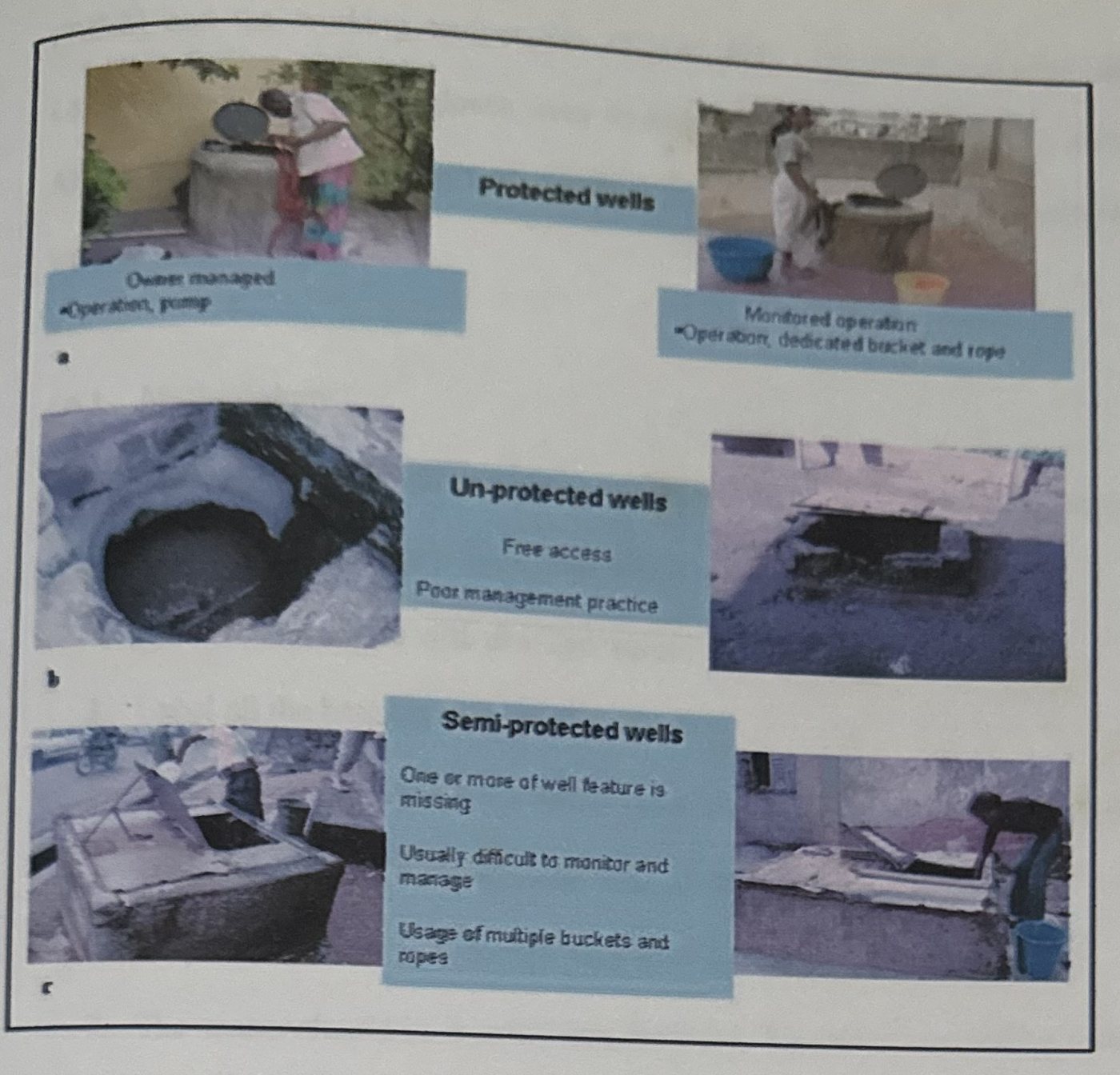
Oluwasanya (2009) noted three types of access to wells namely: restricted (strictly by permission from source owners) access, monitored (owner supervised access) or free access. The author consequently classified self-supply wells into 3 categories of: • Class 1 or Good: Protected well/monitored to restricted access • Class 2 or Fair: Semi-protected/monitored to free access I Class 3 or Poor: Un-protected/free access. (Figure 4-2)
This research employed the aforementioned method of classification for the selected wells.
4.5 Research Constraints
The major obstacles encountered in the course of the project are highlighted here.
- Difficulty in accessing 20 years of Data; either Climatic or Water quality data.
- High Cost of Laboratory Analysis
- Scarcity of Distilled water
4.6 Measurement of Physical Parameters
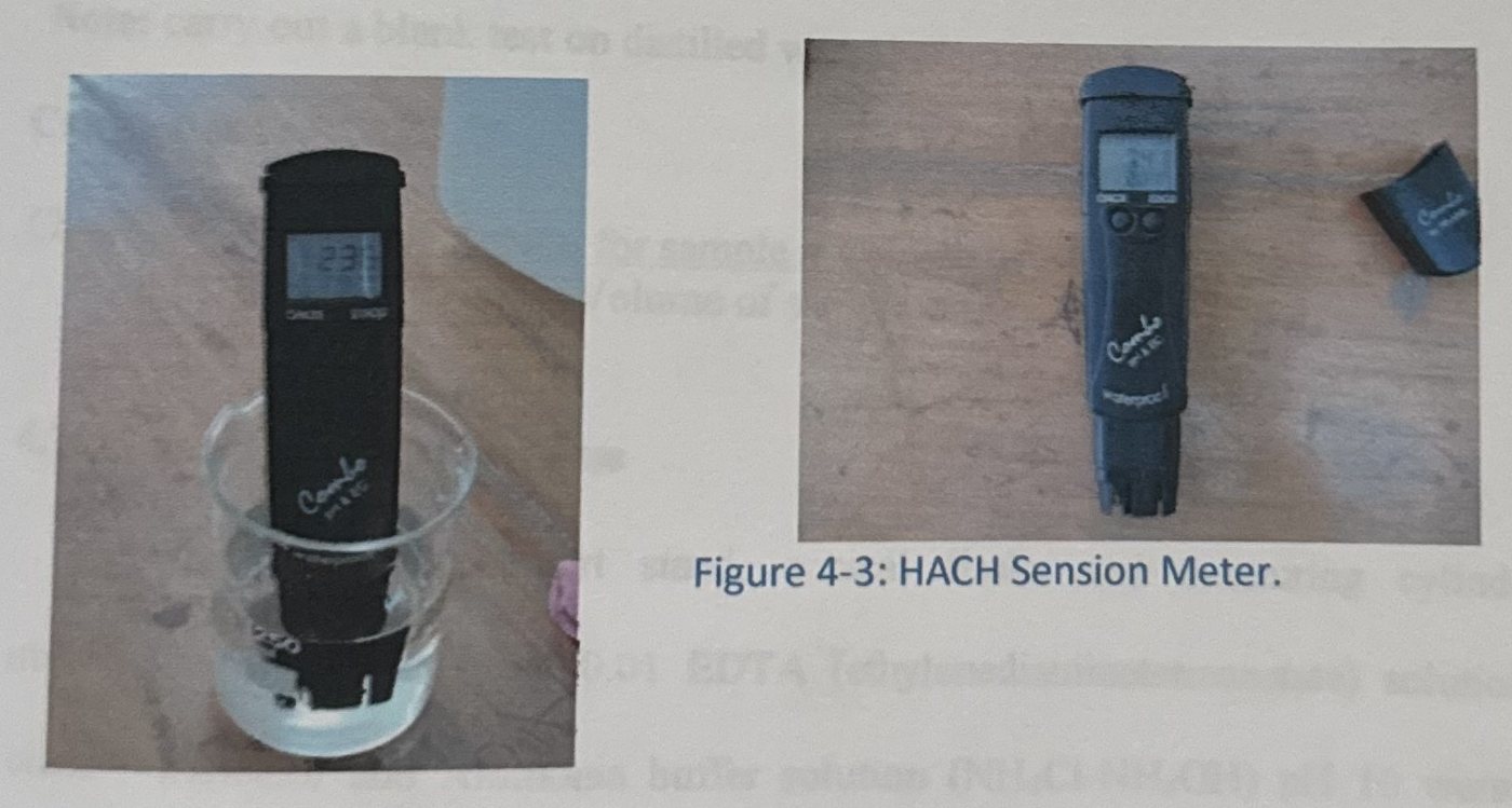
(pH, Electrical Conductivity, Total Dissolved Solids and working Temperature) Physical parameters of water samples were tested using a 4 in 1 HACH sension meter. The HACH sension meter measures the pH, Electrical conductivity [EC], Total dissolved solids [T.D.S] and the working temperature (Figure 4-3). The other materials include beakers, Laboratory coat and Hand gloves worn to ensure safety and reduction of contamination risk. All the materials were rinsed with distilled water including the meter electrode. The beakers were labeled.
4.6.1 Methodology
Laboratory coat and Hand gloves were worn to ensure safety and reduce contamination risk.
- Rinse all the materials to be used with distilled water
- Rinse the electrode with distilled water.
- Label all the beakers to be used.
- Insert the electrode into the buffer solution 4 and then 7, thereafter confirm.
- Dispense 50ml of distilled water into the beaker labeled blank.
- Dispense 50ml of each sample into their respectively labeled beakers
- The sensor should be inserted into the blank, the values read off the dials and recorded.
- The procedure is repeated for the remaining samples and all the other parameters recorded accordingly.
4.7 Measurement of Chemical parameters
4.7.1 Test for Chloride
W.H.O standard for Total Chloride is 250mg/l. Instruments used include Burette, pipette, retort stand, conical flasks, measuring cylinder. Silver Nitrate (AgNO₃), Potassium Chromate (KMnO₄) and Sulphuric acid (H₂SO₄) were the reagents.
Methodology
- Rinse all Glassware to be used with distilled water
- Label all the conical flasks to be used
- Dispense 100ml of each water sample into an already labeled conical flask using a measuring cylinder (using distilled water for the blank)
- Add 2ml of H₂SO₄ using a pipette (the H₂SO₄ acts as a buffer)
- Add 1ml of KMnO₄ solution using a pipette (which acts as an indicator) and gently stir, the solution turns golden yellow on addition.
- Titrate the water samples against the AgNO₃ solution with constant stirring until a slight brick-red color persists.
Note: carry out a blank test on distilled water before using the water samples.
Calculations
Chloride = (Volume of AgNO₃ for sample x Volume of AgNO₃ for Blank x 1000) / Volume of sample
4.7.2 Test for Total Hardness
Burette, pipette, retort stand, conical flasks and measuring cylinder were the instruments employed while 0.01 EDTA (ethylenediaminetetraacetate) solution, Erichrome black-T indicator and Ammonia buffer solution (NH₄Cl-NH₄OH) pH 10 were the reagents used.
Methodology
- Measure 50ml of water sample with a measuring cylinder
- Add 4 drops of Erichrome black-T indicator and mix thoroughly; there should be no color change.
- Add 2ml of buffer solution and mix. The color should change from colorless to purple
- Titrate with the EDTA solution until a blue black solution is obtained (this turns to colorless on standing.)
Calculations
Total Hardness = (1000 x Volume of EDTA) / Volume of sample (100ml)
4.7.3 Test for Nitrates
Nitrate bottles alongside the 6405UV/vis Spectrophotometer were used to carry out the test.
Methodology
- Assemble Nitrate bottles according to the number of sample to be assessed and wash in readiness for the analysis. Allow Nitrate bottles to dry.
- Label the Nitrate bottles accordingly
- Dispense 1ml of each of the samples into the Nitrate bottles.
- Dispense 4ml of distilled water into the Nitrate bottles already containing the sample. Cover the bottles.
- Calibration the spectrophotometer using distilled water as blank.
- Dispensing the sample from the nitrate bottle into the sample container inside the spectrophotometer.
- Read the values from off the dials.
- Repeat steps 6 and 7 for the remaining samples.
4.7.4 Bacteriological and Microbiological Parameters
The Bacteriological and Microbiological indices employed for this research includes; E. Coli or thermo tolerant Coliform count (TE), Clostridium perfringens. Approved tests for total coliform bacteria include the membrane filter, multiple tube fermentation, MPN and MMO- MUG (Colilert") methods. The membrane filter method uses a fine porosity filter which can retain bacteria. The filter is placed in a petri (culture) dish on a pad with growth enrichment media (mEndo) and is incubated for 24 hours at 35 degrees Celsius. Individual bacteria cells which collect on the filter grow into dome-shaped colonies. The coliform bacteria have a gold green sheen, and are counted directly from the dish. Since some other bacteria may develop a similar color, a confirmation test using more specific media is required. The confirmation procedure requires an additional 24 to 48 hours to complete the test for suspected positive total coliform tests.
The MPN procedure involves a multiple tube fermentation technique where three or more decimal dilutions of the sample are inoculated into tubes of broth medium and incubated at a specific temperature and for a specific time. The method is progressive; i.e., first determining the presence of coliforms in the tubes, then determining if these tubes also contain fecal coliforms, and then confirming whether E. coli is present. Based on the number of tubes indicating the presence / absence of the three groups of organisms, the most probable number present can be estimated from a standard statistical MPN table. The MPN (most probable number) method uses a test tube full of media with a smaller inverted test tube inside which captures carbon dioxide gas released from the growth of coliform bacteria. A series of dilutions and replicates are set up, and those producing gas in 24 hours at 35 degrees Celsius are counted. A statistical Analysis is used to determine the most probable number of bacteria cells present.
4.8 Statistical Analysis
4.8.1 Statistical Tools
In view of objective 1, Time series and Correlation were employed as tools in statistical analysis. Graphs were plotted using Microsoft Excel 2010 version. The Total amounts of rainfall and temperature for each year between 1990 and 2012 were plotted together as well as the mean annual temperature for each of the years. The variations depicts rainfall pattern over the years. Only the total amounts of rainfall were used in the time series to identify the trends that exist within it and to establish any change in pattern. Only rainfall was used as Temperature varied only slightly. SPAS 15.0 version was used for this analysis.
Statistical evaluations were carried out using SPAS 15.0 version for the correlation coefficient. The unavailability of continuous data for each location assessed within each of the study areas per year was a limitation. Thus, the following adjustments were made:
- Only the water quality values for the years 1994, 1995, and 2004 were obtainable. Only rainfall amounts for 1994, 1995, and 2004 were used in the correlation analysis. Subsequently, correlation analysis was limited to rainfall data for the selected years.
- The Rainfall amount for 2012 could not be obtained and water quality data for 2011. Rainfall values for 2011 were correlated with water quality values of 2012. The high amount of rain that fell in 2011 (Sub-section 5.3) is expected to have impact on the water quality of 2012.
- The obtained data were taken to represent water quality status in the Abeokuta metropolis. Multiple streams of available water quality data were compressed to aid correlation and reduce errors, as follows:
(i) A mean of all the pH values for all the areas assessed in each of the years was calculated to arrive at a composite value for all the areas assessed. This gives a single representing pH value per year.
(ii) Step I above was repeated for the Electrical conductivity and Nitrates. The result is a single composite value per parameter for each of the year selected.
(iii) A mean of the total amounts of rainfall for the years selected was calculated. The result is a single value used for statistical evaluations.
(iv) A mean of all the values obtained in step I and II above was calculated for all water quality parameters concerned. The result is a single value used for statistical evaluations.
(v) The mean rainfall value was correlated alongside each of the mean values obtained in step IV above to yield a value of significance. The process was repeated for each parameter previously selected.
CHAPTER FIVE: RESULTS AND DISCUSSION
5.0 Introduction
The results obtained from the various laboratory analysis carried out are presented in form of table, histograms and graphs. The results spiked discussions that helped identify and narrow-down the numerous challenges presented by climate change to water quality. The observations, identifiable trends and possible inferences are presented, as well as statistical variations and analysis, forming a basis for the conclusion and recommendation. The samples are identified by their serial numbers. Preliminary water Quality testing and well Classifications are presented in Table 5-1.
About the tables and charts in this chapter. In the printed report the figures are images. Here they are redrawn from the numbers in the annex tables, so every point can be read, checked and downloaded. Some plotted points in the printed figures appear lower than the tabulated values (for example nitrate at samples 9 and 11, and the 2002, 2007 and 2011 rainfall peaks); the tables are used here. Photographs of every printed page that carries a table or figure are listed at the end of the annexes.
Table 5-1: Classifications and Preliminary Examinations
| S/N | Type of water source | Location | Well classification | Colour | Clarity | Potability |
|---|---|---|---|---|---|---|
| 1 | Well | Aba-Olododo Street, Kuto | Protected | Colourless | Clear | Good |
| 2 | Well | Shonibi Street, Onikolobo | Protected | Colourless | Clear | Very Good |
| 3 | Well | Car wash, Asero | Semi-protected | Colourless | Clear | Good |
| 4 | Well | Ake road, Ijemo | Semi-protected | Slightly Milky | Very Slightly Turbid | Fair |
| 5 | Well | Ekundayo Street, Ijeun Titun | Semi-protected | Slightly Milky | Very Slightly Turbid | Fair |
| 6 | Borehole | Mini water works, Ijako Street, Ijemo Agbadu | Protected | Colourless | Clear | Good |
| 7 | Well | Ilogbo Street, Ago-oko | Protected | Colourless | Clear | Good |
| 8 | Well | Tomide Street, Idi-Aba | Protected | Colourless | Clear | Good |
| 9 | Borehole | Laderin Estate, Oke-mosan | Protected | Colourless | Clear | Good |
| 10 | Well | Nepa road, Isabo | Semi-protected | Colourless | Clear | Poor |
| 11 | Well | Iporo-Ake | Semi-protected | Colourless | Clear | Good |
| 12 | Well | Araromi Street, Ita Oshin | Protected | Colourless | Clear | Good |
| 13 | Well | Somorin | Protected | Colourless | Clear | Very Good |
| 14 | Borehole | Keystone Bank, Omida | Protected | Colourless | Clear | Good |
| 15 | Borehole | O.S.H.C Ibara | Protected | Colourless | Clear | Good |
Observations: From Table 5-1, 0% of the sources were un-protected, 3% were semi-protected and 66.7% were protected. [As printed. In the table, 5 of the 15 sources, 33.3%, are classed semi-protected and 10, 66.7%, protected.]
5.1 Physical Parameters
Temperature results of assessed samples are presented in figure 5-1, their Electrical Conductivity obtained are shown in figure 5-2 while figure 5-3 showed the pH results of water samples.
Figure 5-1: mean Temperatures values of the sampled water; WHO standard: Ambient temperature.
Figure 5-2: The mean Electrical Conductivity values of assessed samples; WHO standard: 1000 µScm⁻¹.
Figure 5-3: Mean pH values of self-supply systems in Abeokuta Metropolis; WHO Standard: 6.5–8.5.
NOTE: To convert conductivity of 831 µs/cm at 30 °C to conductivity at 25 °C. Recall, conductivity variation index is 2% per °C. Therefore 2% of 831 µs/cm at 30 °C = [(2/100 × 831) × (30 °C – 25 °C)]. The actual conductivity value at 25 °C is = 831 µs/cm – 83.1 = 747.9 µs/cm.
Observations
- From figure 5-1, all the samples were within ambient temperature.
- With the exception of samples 4 and 10, the electrical conductivity values are NOT above the WHO standards but are fairly high relative to the other samples (Figure 5-2). The observation suggests Microbial and/ or Nutrient load according to CEPIS (2008).
- From figure 5-3, though No sample exceeded the WHO standard for pH, samples 3, 6, 12, 13, and 15 decreased while samples 4, 7, 9, 12 and 14 increased.
5.2 Chemical parameters
Chloride Concentrations are presented in figure 5-4, the Hardness obtained are shown in figure 5-5 while figure 5-6 showed the Nitrates results of water samples.
Figure 5-4: Mean Chloride values of Self supply systems in Abeokuta Metropolis; WHO standard: 250mg/l.
Figure 5-5: Mean Hardness values of Assessments in Abeokuta Metropolis; WHO standard: 150mg/l.
Figure 5-6: Nitrates value of Self supply systems in Abeokuta Metropolis; WHO standard: 50mg/l.
NOTE: Sample 1 in the graphs above represents Blank. [In the printed Figures 5-4 and 5-5 the first position is the blank, so the sample numbers quoted in observations 1 and 2 below are one higher than the sample numbers in the tables and in the chart above: the one sample over the chloride limit is sample 4 in Table A3-1, and the hardness values are lowest at samples 9, 12, 14 and 15.]
Observations
- From figure 5-4, only sample 5 exceeded the WHO standard (250mg/l). This reflects the presence of chlorides in that location.
- From figure 5-5, Sample 10, 13 15 and 16 had the lowest value, while sample 2, 6, 8, 11, 12 and 14 had higher values exceeding the WHO standard (150mg/l).
- From figure 5-6, the results show the presence of nitrates and give an insight into the source and pathways of pollutants in the locations. The samples that exceed the WHO standards contained microbial load, thus confirming microbial results (ANNEX; Table A3-3 and A3-4).
5.3 Microbial Parameters
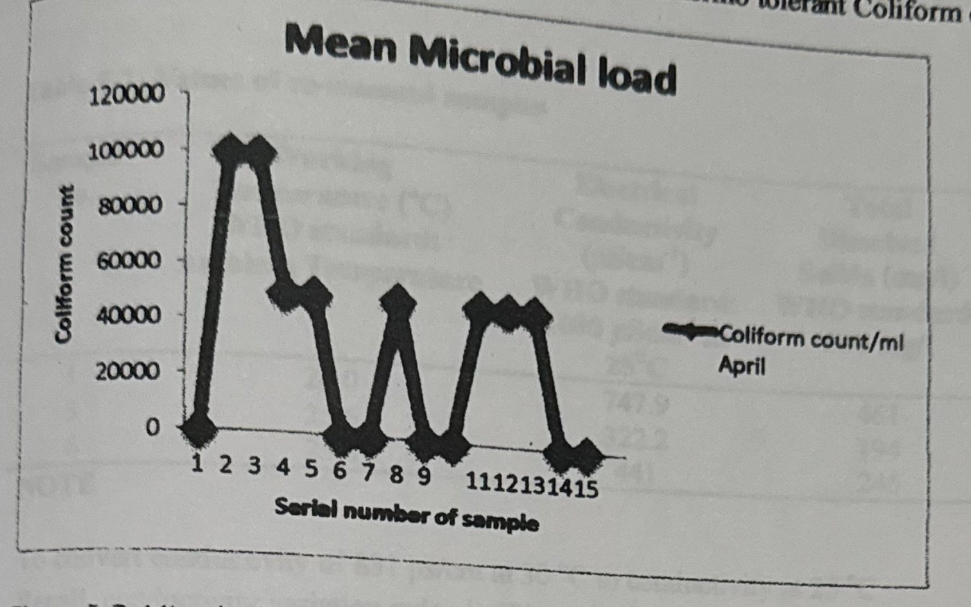
Figure 5-7 shows the results of the mean microbial load for samples collected. WHO Standard: Total Coliform Count: 10cfu/mL. Thermo tolerant Coliform or E.coli: NIL.
Observations
Samples 1, 6, 7, 9, 10, 14, and 15 did not contain any form of pathogens all through the period of analysis. Samples 1, 7 and 10 are wells while 6, 9, 14, and 15 are boreholes. The above graph illustrates the similarities between the Microbial and Nitrate load (Sub-section 2.5.3). Water samples were left on standing after laboratory analysis. It was interested to note that:
- After Forty-six (46) days of the initial assessment, Prominent and accelerated algal growth was seen in all the initial 15 samples assessed in March with the exception of samples 2 and 12.
- After the second and third assessments, similar algal growth occurred in the April and May Assessments though with varying lengths of days-interval.
Upon further observation, Three (3) of the samples that were initially assessed in March; samples 1, 3 and 6 (those with the most prominent and accelerated growth) were selected for re-assessment. Their physical parameters were re-assessed. The results are presented in Table 5-2.
Table 5-2: Values of re-assessed samples
| Sample No. | Working temperature (°C), WHO standard: ambient temperature | Electrical conductivity (µScm⁻¹) at 25 °C, WHO standard: 1000 µScm⁻¹ | Total dissolved solids (mg/l), WHO standard: 500 mg/l | pH, WHO standard: 6.5–8.5 |
|---|---|---|---|---|
| 1 | 26.0 | 747.9 | 461 | 9.47 |
| 3 | 25.6 | 322.2 | 194 | 9.96 |
| 6 | 25.8 | 441 | 245 | 9.57 |
NOTE: To convert conductivity of 831 µs/cm at 30 °C to conductivity at 25 °C. Recall, conductivity variation index is 2% per °C. Therefore 2% of 831 µs/cm at 30 °C = [(2/100 × 831) × (30 °C – 25 °C)] = 70 [sic]. The actual conductivity value at 25 °C is = 831 µs/cm – 83.1 = 747.9 µs/cm.
From table 5-2, the Electrical Conductivity and the Total Dissolved Solids values dropped relative to the initial values that were obtained in-situ. The pH values of each of the samples containing growth rose above the W.H.O standards. Hence, the samples are alkaline in nature. Algal growth rate in the samples had fallen and almost tending to nil (Field observations, 2012).
The implication of above observation is that increased algal growth algal growth in water left on standing may be related to climate change. The algae, (identified as red and brown algae respectively), is not poisonous or harmful to man but may cause psychological reactions on sight (a feeling of being poisoned or nausea). This is not a new phenomenon, rather what new is the reduction in the time taken for algal growth to occur (Table 5-3).
Table 5-3: Time Log for Algal growth in samples
| Assessment | Algal growth | Time taken from sample collection (days) | Percentage growth (%) |
|---|---|---|---|
| March Assessment | Yes | 46 | 86.7 |
| April Assessment | Yes | 10 | 80 |
| May Assessment | Yes | 4 | 70 |
5.4 Climatic Data
Figure 5-8: Total Rainfall Data (1990 – 2011) for Abeokuta Metropolis. Source: OORBDA, 2012.
Figure 5-9: Annual mean temperatures (1990 – 2011) for Abeokuta Metropolis. Source: OORBDA; 2012.
The volume of rainfall increased dramatically, the total amount of rainfall for the year 2011 illustrates this (Figure 5-8). There is however, only a consistent gradual decrease in temperature over the assessed period (Figure 5-9). The observation suggests an indirect relationship between precipitation and temperature.
5.5 Statistical Evaluations
5.5.1 Autocorrelations
A value less than 1 implies NIL auto-correlation. Hence, preceding years does not have effect on subsequent ones. Figure 5-10 shows the effect of the variable (rainfall) on itself over the period under assessment. None of the values obtained are greater than or equal to 1. Thus, amount of rainfall in 1990 has no effect on the amount of rains in 1991 and so on up to 2011. Correlation sequences reflect the order in which rainfall and water quality parameters were correlated.
Figure 5-10: Rainfall Auto-correlation.
5.5.2 Correlation of Rainfall and pH
Table 5-4: Descriptive Statistics of Rainfall and pH
| Mean | N (Number of years) | |
|---|---|---|
| Rainfall | 1603.92500 | 4 |
| pH | 6.7575 | 4 |
Table 5-5: Correlation of Rainfall and pH (Correlations)
| Rainfall | pH | ||
|---|---|---|---|
| Rainfall | Pearson Correlation | 1 | .979* |
| Sig. (2-tailed) | .021 | ||
| Number of years assessed | 4 | 4 | |
| pH | Pearson Correlation | .979* | 1 |
| Sig. (2-tailed) | .021 | ||
| Number of years assessed | 4 | 4 |
*. Correlation is significant at the 0.05 level (2-tailed).
5.5.3 Correlation of Rainfall and Nitrate levels
Table 5-6: Descriptive Statistics of Rainfall and Nitrates
| Mean | N (Number of years) | |
|---|---|---|
| Rainfall | 1603.92500 | 4 |
| NO₃ | 26.069171 | 4 |
Table 5-7: Descriptive Statistics of Rainfall and Nitrates (Correlations, as titled in the report)
| Rainfall | NO₃ | ||
|---|---|---|---|
| Rainfall | Pearson Correlation | 1 | .993** |
| Sig. (2-tailed) | .007 | ||
| N | 4 | 4 | |
| NO₃ | Pearson Correlation | .993** | 1 |
| Sig. (2-tailed) | .007 | ||
| N | 4 | 4 |
**. Correlation is significant at the 0.01 level (2-tailed).
5.5.4 Correlation Results and Inference
Table 5-4 shows the result of correlating rainfall and pH, 0.979 significance was obtained. This implies that rainfall has a 97.9 percentile effect on pH. Thus, Climate has a significant effect on pH.
Correlation of rainfall and Nitrates show significance of 0.993 (Table 5-7). The result implies that rainfall has a 99.3 percentile effect on Nitrates. The increasing microbial and/or nutrient load could be attributed to the increasing precipitation events. (Sub-section 2.7.3). Further research is needed to be conducted to prove this. Thus, rainfall has a significant effect on Nitrate content. A direct relationship exists between both.
5.6 Discussion of Results
Ground water discharge plays an important role in maintaining cooler water temperatures in streams; the cooling effect could be reduced as ground water temperatures are expected to warm with increases in air temperature (meisner et al., 1988). A water quality sensitivity analysis for the Grand River in Ontario showed that, in conjunction with nutrient loading, the dissolved oxygen levels in a eutrophic system were more sensitive to changes in water temperature, particularly over-night water temperature, than to changes in flow. Similar relationships were observed during the 1998 and 1999 droughts. Reduction/ control of water temperature pollution may require a higher degree of consideration in the future (minshall, 2000).
CEPTS (2008) concludes that scenarios of climatic change predicted for the region (temperature increasing, decrease of the precipitations and of the flows), added to the anthropic impacts of the future urbanizations, they will impact in the quality of the water, as it is visualized in the watering channel. Although CEPIS (2008) assessed surface water (rivers), the both methods and results obtained are very similar. Thus, confirming the results obtained from laboratory and statistical evaluations.
Kumar (2010) concludes that although climate change has been widely recognized, research on the impacts of climate change on the groundwater system is relatively limited. The reasons may be that long historical data are required to analyze the characteristics of climate change. These data are not always available. Also, the driving forces that cause such changes are yet unclear. The climatic abnormality may occur frequently and last for a period of time. The conclusion of R. D. Singh serves as necessary backing that further research is needed for confirmation (Sub-section 5.4.2).
Finally, Adverse impacts of climate change on groundwater resources are expected, including changes in recharge rates, and decreased long term groundwater storage. Overall, however, groundwater is expected to be relatively unaffected by the climate change due to its buffering capacity. (Chapter 7; Groundwater and Climate Change).
The results presented in this study, therefore agrees that Climate change has Impacts on water quality of Self-supply systems.
CHAPTER SIX: CONCLUSION AND RECOMMENDATIONS
This chapter begins with a restatement of research objectives, shows how and to what extent each objective has been fulfilled. It concludes with a series of recommendations on the impacts of future climate change. The research objectives include:
- Assessment of climatic conditions (precipitation and temperature) in the study area between 1990 and
- 2011.
- Assessment of Self-Supply System water quality variation (physical, chemical and microbiological) with climatic data in the study area between 1990 and
- 2011.
- Identification and classification of climatic impacts (if any) on the quality on Self-Supply Systems within the study areas.
- Assessment of Self-supply systems.
- Recommendation of appropriate adaptation approaches to water quality management.
6.1 Review of Objectives
Objective #1
There was a significant increase in rainfall in 2011. Hence, Climate change exists within the Study area.
Objectives #2, #3 and #4
From Laboratory and statistical results, pH and Nitrate content were identified as pathways for impacts of Climate change. Rainfall affects pH and Nutrient (Nitrate) levels directly. Algae grow faster in water from self- supply systems due to increase in nutrient levels and slight reduction in groundwater temperature. Hence, Climate change does have effect on the water quality status of self-supply systems.
6.2 Recommendations
In Most of the private residential houses, self - supply well water is consumed or fetched on demand (i.e, as at when needed). This is not always the case as a larger majority prefers to store water. Water storage cannot be eliminated as it helps to be prepared against power failures, drudgery of hauling buckets of water and emergencies. (Emergencies such as having a pressing need for water at odd hours of the day or in unfavorable weather conditions such as rain or excessive sun). The field observation from the study however, revealed the occurrence of algae growth in stored water. Water from self-supply systems (wells and boreholes) should not be left standing for too long; maximum of 2-4 days before use or consumption is recommended and where possible should be consumed on demand. Consuming water on demand or with minimal storage reduces the risk of algal growth.
References
Allan Konopkat and Thomas D. Brock (1978): Effect of Temperature on Blue-Green Algae (Cyanobacteria) in Lake Mendota Department of Bacteriology, University of Wisconsin, Madison, Wisconsin 53706 pp.5
BGR, 2007: Strategies for the Sustainable Management of Non-renewable Groundwater Resources.
Castro E.D 2009: Effect of Agricultural wastes and pollution on ground water deposit in some selected areas of Abeokuta, Ogun State Nigeria. Unpublished project thesis; Department of Water Resources Management and Agrometereology; Federal University of Agriculture, Abeokuta Nigeria.
Center of Excellence for Great Lakes and Human Health 2005: Harmful Algal Blooms in the Great Lakes. Available at http://www.glerl.noaa.gov/res/Centers/HumanHealth/hab/EventResponse
Climate change and Drinking water 2008: Drinking water research; volume 18, number 2, Chapter 2.
DeZuane, John 1997: Handbook of Drinking Water Quality (2nd ed.); John Wiley and Sons. ISBN 0-471-28789-X.
E. O. Orebiyi, et al, 2010: Assessment of Pollution Hazards of Shallow Well Water in Abeokuta and Environs, Southwest, Nigeria; American Journal of Environmental Sciences. 50.56 Volume 6, Issue 1 Pages 50-56
FMW 2004: Federal Ministry of Water Resources Records
Google Images 2012, Available at www.google.com
Guidelines to BSc Project (0056) 2012: Birkbeck, University Of London School of Earth Sciences; pp. 16
Great lakes Regional Assessment group, 2000: Preparing for a changing climate: the potential consequences of Climate variability and change/great lakes overview. P.J. Sousounis, and J.M Bisanz. (eds.). University of Michigan, Ann Arbor, mi.
Groundwater and Climate Change 2002: No Longer the Hidden Resource; IGES White paper
Hyelni H.B 1994: Study of the chemical and Microbiological Characteristics of shallow wells and streams in Abeokuta, Ogun State. Nigeria Unpublished project thesis; Department of Water Resources Management and Agrometereology; Federal University of Agriculture, Abeokuta Nigeria.
IPCC 1996: Impacts, Adaptations and Mitigation of Climate change: scientific-technical analyses. (eds.). Cambridge university press, Cambridge: 1-18.
IPCC 1997: The Regional Impacts of Climate change: An Assessment of Vulnerability. (eds.). Cambridge University Press, Cambridge, 253-330.
London, Cambridge Univ. Press. IPCC 1998: The Regional Impacts of Climate Change: An Assessment of Vulnerability,
IPCC 2001: Climate change 2001: The scientific basis. Summary For policymakers and technical summary of the working group report. WMO and UNEP, 98pp.
IPCC 2008: Climate Change andWater. IPCC Technical Paper VI; Available at: http://www.IPCC.ch/pdf/technical-papers/climate-change-water-en.pdf
IWRM 2004: For sustainable use of water; Ministry of Agriculture, Nature and Food Quality, the Netherlands. W.B Snellen and A. Schrevel (Alterra) Wageningen
Jenny T. et al; 2010: Groundwater, self-supply and poor urban dwellers: A review with case studies of Bangalore and Lusaka
JMP (2005), Water for life: making it happen. Joint monitoring program for water supply and sanitation, WA 675, WHO/UNICEF, New York
JMP (2008), Progress on Drinking water and Sanitation: Special focus on sanitation, 2008 Report, ISBN 978 92 806 4313 8, WHO/UNICEF, New York
Kilanko G.O 1995: Heavy Metals Concentrations in Groundwater in Ogun State, Nigeria. Unpublished project thesis; Department of Water Resources Management and Agrometereology, Federal University of Agriculture, Abeokuta Nigeria.
NIGERIAN INDUSTRIAL STANDARD 2007; Nigerian Standard for Drinking Water Quality; NIS 554
Martins, O., Ajayi, O. and Idowu, O. A. (2000), Factors influencing yields of boreholes in Basement Complex aquifers of South-wester Nigeria, Nigeria Journal of Science, Vol. 34, pp. 295-300.
Microsoft Encarta 2009: Microsoft Encarta and Student Edition.
Morawo O 1991: Chemical Characteristics of Shallow wells in Abeokuta Metropolis: Unpublished project thesis; Department of Water Resources Management and Agrometereology, Federal University of Agriculture, Abeokuta Nigeria.
Onakomaiya, S. O., Oyesiku, K. and Jegede, F. J. (1992), Ogun State in maps, Rex Charles Publication, Nigeria
Oluwasanya G.O.K. 2009: Better Safe than Sorry: Towards Appropriate Water Safety Plans for Urban Self Supply Systems. School of Applied Sciences, Cranfield University; pp 587
OORBDA 2012: Ogun-Osun River Basin Development Authority, Hydrology Department records
Oyawoye M. O 1964: The Geology of Nigerian Basement Complex, Department of Mineral and Geology, pages 87 - 102.
R. D. Singh & C. P. Kumar, 2010: National Institute of Hydrology Roorkee - 247667 (Uttarakhand)
Roberto Bachi 2008: Graphical methods for presenting statistical data: Progress and problems Hebrew University (Israel) pp. 17
Roger C and Alan MacDonald, 2009: What will climate change mean for groundwater supply in Africa? Background Note, pp:4
Sangodoyin, A. Y. 1993: Considerations on contamination of groundwater by waste disposal systems in Nigeria, Environmental Technology, Vol. 14, pp. 957-964
Seamus Collins 2000: Hand dug wells; Series of manuals on Drinking water supply; Vol. 5
Shahbaz Khan; Herbert H.G Serenije, Siegfried Demuth & Pierre Hubert (2010); Hydro complexity: New tools for Solving wicked water Problems. Pages 58 - 70, 233.
Stella McGourty 2006: An investigation into the potential of Household Water Treatment for users of hand dug wells in Busia, Uganda. M.Sc Water Management Community Water Supply, Institute of Water and Environment, Cranfield University
Stuart, M.E., Gooddy, D.C.; Bloomfield, J.P.; Williams, A.T. 2011: A review of the impact of climate change on future nitrate concentrations in groundwater of the UK. Science of the Total Environment, 409 (15). 2859-2873.
Shittu, O.B., et al 2008: Physico-Chemical and Bacteriological Analyses of Water Used for Drinking and Swimming Purposes in Abeokuta, Nigeria; Department of Microbiology, Federal University of Agriculture, Abeokuta, Nigeria African Journal of Biomedical Research, Vol. 11 (2008); 285 - 290 ISSN 1119 - 5096 © Ibadan Biomedical Communications Group.
WHO 2011: Guidelines for Drinking-water Quality Fourth Edition pp. 564.
Wikipedia 2011: Available at www.wikipedia.com
Annexes
Annex 1
Table A1-1: 20 years Climatic Data for Abeokuta Metropolis (Source; OORBDA) Rainfall in mm. Monthly rainfall for 1990 to 2011.
| Year | JAN | FEB | MAR | APR | MAY | JUN | JUL | AUG | SEP | OCT | NOV | DEC | Total rainfall (mm) |
|---|---|---|---|---|---|---|---|---|---|---|---|---|---|
| 1990 | – | 4.9 | 5.2 | 128.4 | 146.2 | 226.4 | 338.5 | 74.9 | 187.1 | 101.5 | 10.7 | 112.3 | 1336.1 |
| 1991 | 6.3 | 111.1 | 109.3 | 118.2 | 70.4 | 81.3 | 273.5 | 127.5 | 167.4 | 98.0 | 2.2 | – | 1165.2 |
| 1992 | – | – | 4.5 | 102.2 | 218.8 | 134.6 | 156.9 | 69.2 | 343.9 | 110.4 | 5.1 | – | 1145.6 |
| 1993 | – | 32 | 92.4 | 39.3 | 163.0 | 185.6 | 98.0 | 37.4 | 148.7 | 134.8 | 4.9 | 5.1 | 941.2 |
| 1994 | 25.8 | 2.2 | 89.9 | 53.7 | 133.0 | 104.6 | 213.3 | 12.5 | 183.9 | 206.7 | 12.4 | – | 1038.0 |
| 1995 | – | 20.8 | 123.0 | 103.8 | 110.0 | 213.7 | 200.1 | 208.0 | 126.2 | 122.2 | 16.9 | – | 1244.7 |
| 1996 | – | 42.3 | 70.3 | 75.1 | 80.1 | 132.1 | 218.6 | 193.1 | 301.1 | 141.9 | – | – | 1254.6 |
| 1997 | 1.5 | – | 129.5 | 284.4 | 134.3 | 218.4 | 51.0 | 111.1 | 79.9 | 174.9 | 13.3 | 35.0 | 1233.5 |
| 1998 | – | – | 19.8 | 123.5 | 176.0 | 168.6 | 55.7 | 48.7 | 178.8 | 82.8 | 18.6 | 23.5 | 896.0 |
| 1999 | 32.8 | 32.2 | 48.68 | 43.1 | 66.8 | 121.0 | 344.3 | 155.7 | 80.2 | 78.1 | 2.6 | 32 | 1008.7 |
| 2000 | 3.4 | – | 110.8 | 31.1 | 74.2 | 140.4 | 68.5 | 267.1 | 204.5 | 48.4 | – | – | 948.4 |
| 2001 | 2.6 | 8.6 | 80.0 | 105.0 | 154.3 | 135.9 | 135.5 | 57.4 | 199.3 | 54.5 | 17.4 | 0.0 | 950.5 |
| 2002 | – | 2.7 | 389.1 | 136.9 | 134.9 | 137.5 | 325.5 | 110.1 | 148.2 | 297.0 | 54.5 | – | 1736.5 |
| 2003 | 12.3 | 25.7 | – | 161.5 | 40.6 | 293.1 | 191.7 | 76.5 | 286.7 | 91.6 | 27.0 | – | 1206.7 |
| 2004 | 15.3 | 20.4 | 75.2 | 83.2 | 233.7 | 145.2 | 130.8 | 73.8 | 172.0 | 163.1 | – | – | 1112.7 |
| 2005 | – | – | 120.4 | 20.8 | 110.2 | 126.2 | 213.7 | 202.1 | 89.3 | 170.0 | 24.0 | 17.0 | 1093.7 |
| 2006 | – | 34.4 | 68.2 | 37.4 | 127.7 | 130.4 | 314.0 | 200.0 | 280.3 | 96.0 | 62.8 | – | 1351.2 |
| 2007 | – | – | 69.5 | 71.4 | 231.2 | 163.5 | 300.7 | 777.6 | 212.1 | 103.5 | 16.4 | – | 1945.9 |
| 2008 | – | – | – | 8.9 | 130.2 | 168 | 8.2 | 192.7 | 126.5 | 120.1 | – | 16.2 | 770.8 |
| 2009 | – | – | 96.0 | 101.0 | 124.0 | 140.0 | 160.0 | 162.1 | 151.6 | 180.1 | 64.6 | 10.4 | 1189.8 |
| 2010 | – | 8.6 | 10.2 | 97.9 | 99.0 | 98.0 | 300.1 | 252.1 | 210.0 | 142.8 | 15.2 | – | 1234.0 |
| 2011 | – | 487.6 | 165.0 | 100.3 | 152.8 | 134.2 | 678.4 | 710.1 | 230.9 | 361.0 | – | – | 3020.3 |
| Monthly total | 100.0 | 835.5 | 1876.9 | 2027.1 | 2911.4 | 3398.7 | 4777 | 4119.7 | 4108.6 | 3079.4 | 368.6 | 251.5 | 27824.1 |
| Monthly mean | 12.5 | 59.53 | 93.85 | 92.14 | 132.34 | 154.48 | 217.14 | 187.26 | 186.75 | 139.97 | 21.68 | 27.94 | 1264.73 |
NOTE: "–" implies Not Available.
Table A1-2: 20 years Mean temperature for Abeokuta Metropolis (Source; OORBDA) Mean monthly temperature in °C.
| Year | JAN | FEB | MAR | APR | MAY | JUN | JUL | AUG | SEP | OCT | NOV | DEC | Mean annual temperature (°C) |
|---|---|---|---|---|---|---|---|---|---|---|---|---|---|
| 1990 | 30.6 | 30.5 | 32.5 | 30.1 | 29.0 | 29.1 | 27.0 | 25.6 | 27.6 | 28.1 | 29.9 | 27.9 | 29.0 |
| 1991 | 29.0 | 30.9 | 30.4 | 28.5 | 29.1 | 28.1 | 27.7 | 25.3 | 25.5 | 25.4 | 29.1 | 28.5 | 27.9 |
| 1992 | 27.2 | 30.6 | 31.8 | 31.7 | 27.9 | 25.5 | 24.1 | 23.8 | 24.6 | 27.5 | 27.9 | 29.4 | 27.7 |
| 1993 | 29.6 | 31.5 | 30.9 | 31.6 | 30.5 | 28.5 | 27.1 | 27.4 | 28.9 | 32.1 | 32.9 | 33.0 | 30.3 |
| 1994 | 33.4 | 36.6 | 35.9 | 35.4 | 33.5 | 32.8 | 32.7 | 33.4 | 34.8 | 34.0 | 33.6 | 34.2 | 34.2 |
| 1995 | 35.6 | 36.4 | 36.1 | 36.2 | 34.9 | 33.6 | 32.2 | 32.2 | 33.0 | 34.5 | 35.8 | 27.9 | 34.0 |
| 1996 | 26.4 | 27.3 | 26.8 | 25.8 | 25.6 | 30.2 | 28.9 | 31.0 | 30.1 | 32.6 | 33.6 | 34.7 | 29.4 |
| 1997 | 34.8 | 35.7 | 34.6 | 33.3 | 32.6 | 31.4 | 31.3 | 31.4 | 32.6 | 33.0 | 35.8 | 37.5 | 33.7 |
| 1998 | 33.8 | 40.2 | 40.2 | 37.4 | 31.7 | 24.7 | 22.3 | 20.6 | 20.1 | 21.7 | 24.5 | 23.8 | 28.4 |
| 1999 | 24.9 | 24.4 | 24.9 | 24.1 | 23.5 | 22.8 | 20.5 | 19.9 | 20.1 | 21.8 | 23.5 | 24.1 | 22.9 |
| 2000 | 25.5 | 24.8 | 27.22 | 25.5 | 24.7 | 24.0 | 23.9 | 23.8 | 23.6 | 24.6 | 25.1 | 26.3 | 24.9 |
| 2001 | 25.6 | 26.2 | 26.8 | 25.6 | 25.0 | 24.2 | 23.8 | 26.5 | 20.6 | 21.6 | 21.4 | 22.0 | 24.1 |
| 2002 | 23.9 | 24.3 | 23.3 | 20.7 | 21.4 | 20.9 | 21.0 | 19.0 | 19.5 | 19.5 | 22.8 | 22.6 | 21.6 |
| 2003 | 23.3 | 24.4 | 26.0 | 27.3 | 22.3 | 22.2 | 21.2 | 21.2 | 21.8 | 22.7 | 27.1 | 23.1 | 23.5 |
| 2004 | 24.1 | 25.3 | 25.4 | 23.8 | 23.1 | 22.3 | 21.3 | 21.2 | 21.9 | 22.8 | 23.4 | 23.5 | 23.2 |
| 2005 | 24.1 | 25.3 | 36.1 | 33.6 | – | – | – | – | – | – | – | – | 29.8 |
| 2006 | – | – | – | – | – | – | – | 26.0 | 26.0 | 25.5 | 25.7 | 25.7 | 25.7 |
| 2007 | 26.1 | 28.0 | 28.7 | 28.4 | 25.7 | 26.2 | 26.9 | 31.5 | 28.6 | 26.2 | 26.7 | 25.8 | 27.4 |
| 2008 | 24.9 | 26.1 | 26.8 | 27.3 | 27.3 | 26.7 | 25.6 | 25.5 | 26.4 | 26.3 | 26.4 | 26.5 | 26.3 |
| 2009 | 26.3 | 26.0 | 26.4 | 26.2 | 26.1 | 26.0 | 26.4 | 26.2 | 24.0 | 26.4 | 26.1 | 26.1 | 26.0 |
| 2010 | 29.7 | 30.3 | 29.7 | 31.7 | 30.65 | 31.8 | 31.8 | 31.6 | 31.7 | 32.2 | 37.0 | 32.0 | 32.0 |
| 2011 | 30.3 | 31.0 | 30.5 | 32.1 | 31.7 | 30.8 | 31.8 | 31.1 | 31.1 | 30.2 | 29.8 | 29.7 | 30.8 |
| Monthly total | 589.1 | 615.8 | 631.0 | 616.3 | 556.2 | 541.8 | 527.5 | 554.2 | 552.5 | 568.7 | 598.1 | 584.3 | 530.7 |
| Monthly mean | 28.1 | 29.3 | 30.0 | 29.3 | 27.8 | 27.0 | 26.3 | 26.4 | 26.3 | 27.0 | 28.5 | 27.8 | 27.9 |
NOTE: "–" implies Not Available.
Annex 2
Table A2-1: Water Quality Status of self-supply systems (wells and boreholes) for 1994 & 1995
| Location | pH | Electrical conductivity (µs/cm) at 25 °C | NO₃²⁻ (mg/l) |
|---|---|---|---|
| TOTORO | 5.9 | 748.8 | 1.0 |
| ABOABA | 7.3 | 495 | 5.0 |
| AMOLASO | 5.6 | 592.5 | 13.0 |
| ITORI-ODO | 6.2 | 1014.3 | 12.0 |
| IGBORE | 6.1 | 834.3 | 20.0 |
| KOBITI | 7.6 | 981.9 | 5.0 |
| ASERO | 5.4 | 301.5 | 10.0 |
| ISALE AKE | 7.3 | 278.1 | 2.0 |
| LANTORO | 5.1 | 199.8 | 2.0 |
| IJAIYE | 8.2 | 692.1 | 4.0 |
| IJEUN TITUN | 7.5 | 235.8 | 4.0 |
| OKE-IJEUN | 7.7 | 986.4 | 23.0 |
| AGO-OKO | 7.2 | 652.5 | 20.0 |
| LAFENWA | 7.2 | 824.4 | 2.0 |
| KUTO | 6.4 | 458.1 | 10.0 |
| AKOMOJE | 5.4 | 219.6 | 1.0 |
| ILAWO | 7.3 | 710.1 | 24.0 |
| ODO ERAN | 7.2 | 225 | 41.3 |
| ODEDA | 6.7 | 447 | 14.2 |
| MEAN VALUES | 6.7 | 573.57 | 11.23 |
NOTE: To convert conductivity of 832 µs/cm at 30 °C to conductivity at 25 °C. Recall, conductivity variation index is 2% per °C. Therefore 2% of 832 µs/cm at 30 °C = [(2/100 × 832) × (30 °C – 25 °C)]. The actual conductivity value at 25 °C is = 832 µs/cm – 83.1 = 748.8 µs/cm.
Source: Hyelni H.B (1994): Study of the chemical and Microbiological Characteristics of shallow wells and streams in Abeokuta, Ogun State Nigeria, Unpublished B.Sc. Dissertation in the Department of Water Resources Management and Agrometereology; Federal University of Agriculture, Abeokuta Nigeria.
Kilanko G.O (1995): Heavy Metals Concentrations in Groundwater in Ogun State, Nigeria, Unpublished B.Sc. Dissertation; in the Department of Water Resources Management and Agrometereology; Federal University of Agriculture, Abeokuta Nigeria.
Table A2-2: Water Quality Status of self-supply systems (wells and boreholes) for 2004
| Location | Temperature (°C) | pH | Electrical conductivity (µs/cm) at 25 °C | Total hardness (mg/l) | Cl²⁻ (mg/l) | NO₂⁻ (mg/l) | Coliform count (CFU/100ml) |
|---|---|---|---|---|---|---|---|
| SOMORIN | 29 | 6.00 | 78.48 | 28 | 30 | 2.01 | 52 |
| OLOKEMEJI | 28.5 | 6.21 | 242.1 | 62 | 60 | 3.21 | 19 |
| CAMP | 29 | 6.20 | 402.3 | 100 | 84 | 4.31 | 21 |
| OSEILE | 28 | 7.20 | 830.7 | 296 | 140 | 7.22 | 50 |
| ODEDA | 29 | 7.60 | 1138.5 | 440 | 180 | 6.21 | 42 |
| OLODO | 38 | 7.40 | 379.8 | 324 | 80 | 3.50 | 34 |
| UNAAB | 28 | 7.60 | 285.3 | 146 | 35 | 4.23 | 15 |
| ALABATA | 28.5 | 6.30 | 436.4 | 282 | 92 | 5.21 | 25 |
| OLUGBO | 29.5 | 6.70 | 219.6 | 220 | 52 | 4.21 | 8 |
| OPEJI | 29 | 7.51 | 207.9 | 260 | 46 | 3.62 | 74 |
| KUTO | – | 6.41 | 458.1 | 160 | 54 | – | >160 |
| QUARRY-ROAD | – | 5.44 | 773.1 | 230 | 96 | – | >160 |
| ISABO | – | 7.32 | 455.4 | 145 | 48 | – | 70 |
| OKE-SHOKORI | – | 7.31 | 495 | 160 | 44 | – | >160 |
| IJAYE | – | 8.24 | 692.1 | 170 | 88 | – | 90 |
| LANTORO | – | 5.14 | 22.2 | 60 | 28 | – | 50 |
| LAFENWA | – | 7.24 | 199.8 | 190 | 98 | – | >160 |
| ASERO | – | 5.42 | 301.5 | 90 | 48 | – | >160 |
| IBEREKODO | – | 5.41 | 219.6 | 70 | 19 | – | >160 |
| IGBORE | – | 6.12 | 834.3 | 210 | 140 | – | >160 |
| IPORO-AKE | – | 7.31 | 278.1 | 100 | 30 | – | >160 |
| ONIKOLOBO | – | 6.22 | 828.0 | 300 | 150 | – | 20 |
| IJAYE KUKUDI | – | 6.24 | 774.0 | 120 | 82 | – | >160 |
| MEAN VALUES | 6.63 | 493.65 | 4.37 | 87.39 |
NOTE: "–" implies Not Available. To convert conductivity of 87.2 µs/cm at 30 °C to conductivity at 25 °C. Recall, conductivity variation index is 2% per °C. Therefore 2% of 87.2 µs/cm at 30 °C = [(2/100 × 87.2) × (30 °C – 25 °C)]. The actual conductivity value at 25 °C is = 87.2 µs/cm – 8.72 = 78.48 µs/cm.
Source: Adeniyi A. O (2004): An Assessment of water quality of Self-supply systems in Odeda local government area of Ogun state Nigeria, Unpublished B.Sc. Dissertation in the Department of Water Resources Management and Agrometereology; Federal University of Agriculture, Abeokuta Nigeria.
Annex 3
Table A3-1: Water Quality Parameters of Self supply systems in Abeokuta Metropolis for the Year 2012
| S/N | Type of system | Working temperature (°C, at time of collection) | Electrical conductivity (µScm⁻¹) | Electrical conductivity (µScm⁻¹) at 25 °C | pH | Chloride (mg/l) | Hardness (mg/l) | NO₃²⁻ (mg/l) |
|---|---|---|---|---|---|---|---|---|
| 1 | Well | 29.73 | 937.60 | 843.84 | 7.05 | 132.00 | 187.30 | 139.51 |
| 2 | Well | 29.00 | 323.30 | 290.97 | 7.16 | 58.60 | 113.00 | 185.37 |
| 3 | Well | 29.83 | 477.30 | 429.97 | 6.69 | 63.00 | 140.00 | 119.02 |
| 4 | Well | 30.00 | 1314.60 | 1183.14 | 7.43 | 295.00 | 163.33 | 52.68 |
| 5 | Well | 30.6 | 849.30 | 764.40 | 6.87 | 153.60 | 260.00 | 121.95 |
| 6 | Borehole | 30.3 | 578.00 | 520.20 | 6.37 | 123.60 | 190.60 | 53.66 |
| 7 | Well | 30.23 | 914.30 | 822.90 | 6.93 | 89.33 | 306.00 | 61.46 |
| 8 | Well | 30.27 | 301.60 | 271.44 | 6.28 | 39.00 | 134.00 | 75.12 |
| 9 | Borehole | 30.13 | 47.30 | 42.57 | 6.79 | 21.60 | 58.00 | 29.27 |
| 10 | Well | 31.00 | 1140.60 | 1026.54 | 6.98 | 110.30 | 262.00 | 40.00 |
| 11 | Well | 30.20 | 783.30 | 704.97 | 6.83 | 93.60 | 230.00 | 140.00 |
| 12 | Well | 29.96 | 287.60 | 258.84 | 7.64 | 15.30 | 30.00 | 77.07 |
| 13 | Well | 29.33 | 747.60 | 672.84 | 7.32 | 60.60 | 220.00 | 15.61 |
| 14 | Borehole | 30.50 | 250.60 | 225.54 | 7.87 | 25.00 | 40.00 | 40.00 |
| 15 | Borehole | 30.83 | 207.30 | 186.57 | 6.72 | 28.30 | 50.00 | 10.73 |
| WHO standard | Ambient temperature | 1000 µScm⁻¹ | 6.5–8.5 | 250 mg/l | 150 mg/l | 50 mg/l |
NOTE: To convert conductivity of 937.6 µs/cm at 30 °C to conductivity at 25 °C. Recall, conductivity variation index is 2% per °C. Therefore 2% of 937.6 µs/cm at 30 °C = [(2/100 × 937.6) × (30 °C – 25 °C)]. The actual conductivity value at 25 °C is = 937.6 µs/cm – 93.76 = 843.84 µs/cm. Source: Field work, 2012.
Table A3-2: Values for Selected Years
| S/N | Year | Annual rainfall per year | Mean pH | Mean electrical conductivity (µScm⁻¹) at 25 °C | Mean nitrates (mg/l) | Mean temperature (°C) |
|---|---|---|---|---|---|---|
| 1 | 1994 | 1038 | 6.7 | 573.57 | 11.23 | 34.2 |
| 2 | 1995 | 1244.7 | 6.7 | 573.57 | 11.23 | 34.2 |
| 3 | 2004 | 1112.7 | 6.63 | 493.65 | 4.37 | 23.2 |
| 4 | 2012 | 3020.3 | 6.99 | 549.61 | 77.43 | 30.8 |
| Overall mean | 1603.93 | 6.75 | 547.6 | 26.06 | 30.6 |
Table A3-3: Water Culture Analysis Result for April 2012 (the report prints "April 21012")
| Code | Culture | Gram stain | Results | Count |
|---|---|---|---|---|
| 1 | No growth | – | – | – |
| 2 | Moderate growth | GPC | Non-pathogenic | <10⁵/ml |
| 3 | Moderate growth | GPC | Non-pathogenic | <10⁵/ml |
| 4 | Moderate growth | GPC | Non-pathogenic | <10⁵/ml |
| 5 | No growth | – | – | – |
| 6 | No growth | – | – | – |
| 7 | No growth | – | – | – |
| 8 | Moderate growth | GPC | Non-pathogenic | <10⁵/ml |
| 9 | No growth | – | – | – |
| 10 | No growth | – | – | – |
| 11 | Moderate growth | GPC | Non-pathogenic | <10⁵/ml |
| 12 | Moderate growth | GPC | Non-pathogenic | <10⁵/ml |
| 13 | No growth | – | – | – |
| 14 | No growth | – | – | – |
| 15 | No growth | – | – | – |
NOTE: GPC: Gram Positive Cocci; implying the presence of non-pathogenic Micro-organisms. Laboratory: Apex Medical Diagnostic Laboratory, Asero, Abeokuta. Medical Laboratory Scientist: Amusan, A. T, M.Sc. (In-view), AIMLS, FMLSCN.
Table A3-4: Water Culture Analysis Result for May 2012
| Code | Culture | Gram stain | Results | Count |
|---|---|---|---|---|
| 1 | No growth | – | – | – |
| 2 | Moderate growth | GPC | Non-pathogenic | – |
| 3 | Moderate growth | GPC | Strept. spp | <10⁵/ml (10) |
| 4 | No growth | – | – | – |
| 5 | Heavy mixed growth | GPC, GNB | Streptococci, coliform bac. | >10⁵/ml (35); 205 CFU/ml |
| 6 | No growth | – | – | – |
| 7 | Moderate growth | GNB | E. coli | 110 CSU/ml |
| 8 | Heavy mixed growth | GPC, GNB | Streptococci, E. coli | >10⁵/ml (39); 185 CFU/ml |
| 9 | No growth | – | – | – |
| 10 | No growth | – | – | – |
| 11 | Heavy mixed growth | GNB | C. perfringens, E. coli | >10⁵/ml (17); 210 CFU/ml |
| 12 | Moderate growth | GPC | Non-pathogenic | – |
| 13 | Heavy mixed growth | GNB | Coliform bac., E. coli | >10⁵/ml (32); 167 CFU/ml |
| 14 | No growth | – | – | – |
| 15 | No growth | – | – | – |
| 16 | No growth | – | – | – |
NOTE: GPC: Gram Positive Cocci; implying the presence of non-pathogenic Micro-organisms. GNB: Gram Negative Baccilli; depicting the presence of pathogenic Micro-organisms. CFU: Coliform Forming Unit, a unit of measurement equivalent to Coliform Count. Laboratory: Apex Medical Diagnostic Laboratory, Asero, Abeokuta. Medical Laboratory Scientist: Amusan, A. T, M.Sc. (In-view), AIMLS, FMLSCN.
Table A3-5: Rainfall statistical Evaluations Series: rainfall.
| Lag | Autocorrelation | Std. error | Box-Ljung value | df | Sig. |
|---|---|---|---|---|---|
| 1 | -.009 | .199 | .002 | 1 | .966 |
| 2 | -.056 | .195 | .086 | 2 | .958 |
| 3 | -.194 | .190 | 1.132 | 3 | .769 |
| 4 | .284 | .185 | 3.491 | 4 | .479 |
| 5 | .167 | .179 | 4.360 | 5 | .499 |
| 6 | -.099 | .174 | 4.682 | 6 | .585 |
| 7 | -.018 | .169 | 4.694 | 7 | .697 |
| 8 | -.022 | .163 | 4.713 | 8 | .788 |
| 9 | .139 | .157 | 5.500 | 9 | .789 |
| 10 | -.076 | .151 | 5.752 | 10 | .836 |
| 11 | -.104 | .144 | 6.275 | 11 | .854 |
| 12 | -.075 | .138 | 6.574 | 12 | .884 |
| 13 | -.168 | .131 | 8.240 | 13 | .828 |
| 14 | -.035 | .123 | 8.323 | 14 | .872 |
| 15 | .012 | .115 | 8.334 | 15 | .910 |
| 16 | -.001 | .107 | 8.334 | 16 | .938 |
| 17 | -.060 | .097 | 8.718 | 17 | .949 |
| 18 | -.127 | .087 | 10.840 | 18 | .901 |
| 19 | -.045 | .075 | 11.201 | 19 | .917 |
| 20 | -.038 | .062 | 11.580 | 20 | .930 |
a. The underlying process assumed is independence (white noise). b. Based on the asymptotic chi-square approximation.
Annex 4
Table A4: Project Schedule
| Time frame | Description of activities carried out |
|---|---|
| Feb 23rd – March 7th | Thesis sketch and prototype |
| March 9th | Scheduling of meetings with project supervisor; Literature review #1; Field work commences; Visit to Abeokuta-south local Government Headquarters; Determination of materials needed for Laboratory analysis and purchase; Identification of Project Aim and objectives |
| March 12th – March 22nd | Literature review #2; Site visits #1 and #2: Location, Determination and Identification of private wells to participate; Determination of sample size and Dates of collection; Determination of water parameters to be assessed |
| March 23rd – April 3rd | Paperwork Review by Project supervisor #1; Literature review #3; Site visit #3: Collection of 1st assessments; Data collection (climatic and water quality); Laboratory analysis of assessments |
| April 4th – May 9th | Paperwork Review by Project supervisor #2; Literature review #4; Site visit #4: Collection of 2nd assessments; Thesis construction and buildup; Laboratory analysis and assessments; Observation and further analysis |
| May 10th – June 9th | Paperwork Review by Project supervisor #3; Literature review #5; Site visit #5: Collection of 3rd set of assessments; Laboratory analysis and assessments; Preparation for Statistical Analysis |
| 10th June | Paperwork Review by Project supervisor #4; Literature review #6; Identification of trends and discussion of results |
| 15th June – 29th | Paperwork Review by Project supervisor #5; Literature review #7; Review of project objectives; Conclusion and recommendations |
| 29th June – 12th July | Paperwork Review by Project supervisor #6 (Chapters 1 – 3); Literature review #8; Statistical Analysis |
| 12th July – 23rd July | Paperwork Review by Project supervisor #7 (Chapters 4 – 6); Literature review #9 |
| 28th July – 30th July | Paperwork Review by Project supervisor #8 (Chapters 1 – 6); Submission of thesis for final assessment |
| 31st July | Project Defence |
In the printed table the dates sit beside the activities; the grouping above follows the position of each date against its first activity.
Annex 5: Nigerian Drinking Water Standards
Table A5-1: Physical / Organoleptic Parameters
| Parameter | Unit | Maximum permitted levels | Health impact |
|---|---|---|---|
| Colour | TCU | 15 | None |
| Odour | – | Unobjectionable | None |
| Taste | – | Unobjectionable | None |
| Temperature | °Celsius | Ambient | None |
| Turbidity | NTU | 5 | None |
Source: NIGERIAN INDUSTRIAL STANDARD 2007; Nigerian Standard for Drinking Water Quality; NIS 554.
Table A5-2: Chemical Parameters
| Parameter | Unit | Maximum permitted | Health impact |
|---|---|---|---|
| Aluminum (Al) | mg/L | 0.2 | Potential Neuro-degenerative disorders |
| Arsenic (As) | mg/L | 0.01 | Cancer |
| Barium | mg/L | 0.7 | Hypertension |
| Cadmium (Cd) | mg/L | 0.003 | Toxic to the kidney |
| Chloride (Cl) | mg/L | 250 | None |
| Chromium (Cr⁶⁺) | mg/L | 0.05 | Cancer |
| Conductivity | µScm⁻¹ | 1000 | None |
| Copper (Cu²⁺) | mg/L | 1 | Gastrointestinal disorder |
| Cyanide (CN⁻) | mg/L | 0.01 | Very toxic to the thyroid and the nervous system |
| Fluoride (F⁻) | mg/L | 1.5 | Fluorosis, Skeletal tissue (bones and teeth) morbidity |
| Hardness (as CaCO₃) | mg/L | 150 | None |
| Hydrogen Sulphide (H₂S) | mg/L | 0.05 | None |
| Iron (Fe+2) | mg/L | 0.3 | None |
| Lead (Pb) | mg/L | 0.01 | Cancer, interference with Vitamin D metabolism, affect mental development in infants, toxic to the central and peripheral nervous systems |
| Magnesium (Mg+2) | mg/L | 0.20 | Consumer acceptability |
| Manganese (Mn+2) | mg/L | 0.2 | Neurological disorder |
Source: NIGERIAN INDUSTRIAL STANDARD 2007; Nigerian Standard for Drinking Water Quality; NIS 554.
Table A5-3: Inorganic Constituents (Contd.)
| Parameter | Unit | Maximum permitted | Health impact |
|---|---|---|---|
| Mercury (Hg) | mg/L | 0.001 | Affects the kidney and central nervous system |
| Nickel (Ni) | mg/L | 0.02 | Possible carcinogenic |
| Nitrate (NO₃) | mg/L | 50 | Cyanosis, and asphyxia („blue-baby syndrome”) in infants under 3 months |
| Nitrite (NO₂) | mg/L | 0.2 | Cyanosis, and asphyxia („blue-baby syndrome”) in infants under 3 months |
| pH | – | 6.5–8.5 | None |
| Sodium (Na) | mg/L | 200 | None |
| Sulphate (SO₄) | mg/L | 100 | None |
| Total Dissolved Solids | mg/L | 500 | None |
| Zinc (Zn) | mg/L | 3 | None |
Source: NIGERIAN INDUSTRIAL STANDARD 2007; Nigerian Standard for Drinking Water Quality; NIS 554.
Notes on this transcription
The annex tables were typed from photographs of the printed pages and every column was checked against the totals and means printed on the same page. Where the print disagrees with itself, the printed value is kept and the difference is listed here.
- Table A1-1. Rainfall columns reproduce the printed monthly totals, and the annual totals reproduce the printed 27,824.1 and mean of 1,264.73. Four rows differ slightly from their printed annual total: the monthly entries for 1997, 2002 and 2010 sum to 0.2, 0.1 and 0.1 mm less than the printed total, and December 1999 is printed "32" although the 1999 total only works with 3.2 (the printed December total, 251.5, includes 32). The printed February total reads 835.5 while the entries sum to 833.5.
- Table A1-2. Every monthly column reproduces its printed total. The printed mean annual temperature differs from the average of the months for 1991 (27.9 printed, 28.1 from the months), 2006 (25.7, 25.8) and 2010 (32.0, 31.7); the printed values are shown.
- Table A2-1. The pH and nitrate means reproduce; the conductivity mean of the 19 values is 573.54 against 573.57 printed.
- Table A2-2. The pH, nitrite and coliform means reproduce (coliform counts of >160 taken as 160). The 23 conductivity values as printed average 458.8 µs/cm, not the 493.65 printed.
- Table A3-1. The nitrate mean, 77.43, reproduces; the pH mean is 7.00 and the conductivity mean 549.65 against 6.99 and 549.61 printed in Table A3-2. The last row of the printed conductivity column repeats 937.60 beside the WHO standard; it is left out here.
- Table A3-2. The 2012 row carries the 2011 rainfall (3,020.3 mm) and mean temperature (30.8 °C), as printed. The 1995 temperature is printed 34.2 where Table A1-2 gives 34.0.
- Table A3-5. The lag 3 autocorrelation is cut off in the photograph; −0.194 reproduces the printed Box-Ljung value.
- Table 5-1. The observation prints 3% semi-protected where the table gives 33.3%.
- Pages photographed twice. Printed page 66 (Table A3-3) and the Annex 4 schedule each appear twice in the scans; one copy of each is kept.
Printed pages
Photographs of the printed pages that carry the tables and figures above, for checking this transcription against the original.
- Report page 42: Table 5-1
- Report page 43: Figures 5-1 and 5-2
- Report page 44: Figure 5-3
- Report page 45: Figures 5-4 and 5-5
- Report page 46: Figure 5-6
- Report page 47: Figure 5-7
- Report page 48: Table 5-2
- Report page 49: Table 5-3, Figures 5-8 and 5-9
- Report page 50: Figure 5-10
- Report page 51: Tables 5-4 and 5-5
- Report page 52: Tables 5-6 and 5-7
- Report page 61: Table A1-1
- Report page 62: Table A1-2
- Report page 63: Table A2-1
- Report page 64: Table A2-2
- Report page 65: Tables A3-1 and A3-2
- Report page 66: Table A3-3
- Report page 67: Table A3-4
- Report page 68: Table A3-5
- Report page 69: Table A4
- Report page 70: Tables A5-1 and A5-2
- Report page 71: Table A5-3